What's the difference and connections between recursion, divide-and-conquer algorithm, dynamic programming, and greedy algorithm? If you haven't made it clear. Doesn't matter! I would give you a brief introduction to kick off this section.
Recursion is a programming technique. It's a way of thinking about solving problems. There're two algorithmic ideas to solve specific problems: divide-and-conquer algorithm and dynamic programming. They're largely based on recursive thinking (although the final version of dynamic programming is rarely recursive, the problem-solving idea is still inseparable from recursion). There's also an algorithmic idea called greedy algorithm which can efficiently solve some more special problems. And it's a subset of dynamic programming algorithms.
The divide-and-conquer algorithm will be explained in this section. Taking the most classic merge sort as an example, it continuously divides the unsorted array into smaller sub-problems. This is the origin of the word divide and conquer. Obviously, the sub-problems decomposed by the ranking problem are non-repeating. If some of the sub-problems after decomposition are duplicated (the nature of overlapping sub-problems), then the dynamic programming algorithm is used to solve them!
Recursion in detail
Before introducing divide and conquer algorithm, we must first understand the concept of recursion.
The basic idea of recursion is that a function calls itself directly or indirectly, which transforms the solution of the original problem into many smaller sub-problems of the same nature. All we need is to focus on how to divide the original problem into qualified sub-problems, rather than study how this sub-problem is solved. The difference between recursion and enumeration is that enumeration divides the problem horizontally and then solves the sub-problems one by one, but recursion divides the problem vertically and then solves the sub-problems hierarchily.
The following illustrates my understanding of recursion. If you don't want to read, please just remember how to answer these questions:
- How to sort a bunch of numbers? Answer: Divided into two halves, first align the left half, then the right half, and finally merge. As for how to arrange the left and right half, please read this sentence again.
- How many hairs does Monkey King have? Answer: One plus the rest.
- How old are you this year? Answer: One year plus my age of last year, I was born in 1999.
Two of the most important characteristics of recursive code: end conditions and self-invocation. Self-invocation is aimed at solving sub-problems, and the end condition defines the answer to the simplest sub-problem.
int func(How old are you this year) {

    // simplest sub-problem, end condition
    if (this year equals 1999) return my age 0;
    // self-calling to decompose problem
    return func(How old are you last year) + 1;

}
Actually think about it, what is the most successful application of recursion? I think it's mathematical induction. Most of us learned mathematical induction in high school. The usage scenario is probably: we can't figure out a summation formula, but we tried a few small numbers which seemed containing a kinda law, and then we compiled a formula. We ourselves think it shall be the correct answer. However, mathematics is very rigorous. Even if you've tried 10,000 cases which are correct, can you guarantee the 10001th correct? This requires mathematical induction to exert its power. Assuming that the formula we compiled is true at the kth number, furthermore if it is proved correct at the k + 1th, then the formula we have compiled is verified correct.
So what is the connection between mathematical induction and recursion? We just said that the recursive code must have an end condition. If not, it will fall into endless self-calling hell until the memory exhausted. The difficulty of mathematical proof is that you can try to have a finite number of cases, but it is difficult to extend your conclusion to infinity. Here you can see the connection-infinite.
The essence of recursive code is to call itself to solve smaller sub-problems until the end condition is reached. The reason why mathematical induction is useful is to continuously increase our guess by one, and expand the size of the conclusion, without end condition. So by extending the conclusion to infinity, the proof of the correctness of the guess is completed.
Why learn recursion
First to train the ability to think reversely. Recursive thinking is the thinking of normal people, always looking at the problems in front of them and thinking about solutions, and the solution is the future tense; Recursive thinking forces us to think reversely, see the end of the problem, and treat the problem-solving process as the past tense.
Second, practice analyzing the structure of the problem. When the problem can be broken down into sub problems of the same structure, you can acutely find this feature, and then solve it efficiently.
Third, go beyond the details and look at the problem as a whole. Let's talk about merge and sort. In fact, you can divide the left and right areas without recursion, but the cost is that the code is extremely difficult to understand. Take a look at the code below (merge sorting will be described later. You can understand the meaning here, and appreciate the beauty of recursion).
void sort(Comparable[] a){
    int N = a.length;
    // So complicated! It shows disrespect for sorting. I refuse to study such code.
    for (int sz = 1; sz < N; sz = sz + sz)
        for (int lo = 0; lo < N - sz; lo += sz + sz)
            merge(a, lo, lo + sz - 1, Math.min(lo + sz + sz - 1, N - 1));
}

/* I prefer recursion, simple and beautiful */
void sort(Comparable[] a, int lo, int hi) {
    if (lo >= hi) return;
    int mid = lo + (hi - lo) / 2;
    sort(a, lo, mid); // soft left part
    sort(a, mid + 1, hi); // soft right part
    merge(a, lo, mid, hi); // merge the two sides
}
Looks simple and beautiful is one aspect, the key is very interpretable: sort the left half, sort the right half, and finally merge the two sides. The non-recursive version looks unintelligible, full of various incomprehensible boundary calculation details, is particularly prone to bugs and difficult to debug. Life is short, i prefer the recursive version.
Obviously, sometimes recursive processing is efficient, such as merge sort, sometimes inefficient, such as counting the hair of Monkey King, because the stack consumes extra space but simple inference does not consume space. Example below gives a linked list header and calculate its length:
/* Typical recursive traversal framework requires extra space O(1) */
public int size(Node head) {
    int size = 0;
    for (Node p = head; p != null; p = p.next) size++;
    return size;
}
/* I insist on recursion facing every problem. I need extra space O(N) */
public int size(Node head) {
    if (head == null) return 0;
    return size(head.next) + 1;
}
Tips for writing recursion
My point of view: Understand what a function does and believe it can accomplish this task. Don't try to jump into the details. Do not jump into this function to try to explore more details, otherwise you will fall into infinite details and cannot extricate yourself. The human brain carries tiny sized stack!
Let's start with the simplest example: traversing a binary tree.
void traverse(TreeNode* root) {
    if (root == nullptr) return;
    traverse(root->left);
    traverse(root->right);
}
Above few lines of code are enough to wipe out any binary tree. What I want to say is that for the recursive
function traverse (root) , we just need to believe: give it a root node
root , and it
can traverse the whole tree. Since this function is written for this specific purpose, so we just need to dump
the left and right nodes of this node to this function, because I believe it can surely complete the task. What
about traversing an N-fork tree? It's too simple, exactly the same as a binary tree!
void traverse(TreeNode* root) {
    if (root == nullptr) return;
    for (child : root->children)
        traverse(child);
}
As for pre-order, mid-order, post-order traversal, they are all obvious. For N-fork tree, there is obviously no in-order traversal.
The following explains a problem from LeetCode in detail: Given a binary tree and a target value, the values in every node is positive or negative, return the number of paths in the tree that are equal to the target value, let you write the pathSum function:
/* from LeetCode PathSum III: https://leetcode.com/problems/path-sum-iii/ */
     root = [10,5,-3,3,2,null,11,3,-2,null,1],
     sum = 8

     10
     / \
     5 -3
     / \ \
     3 2 11
     / \ \
     3 -2 1

     Return 3. The paths that sum to 8 are:

     1. 5 -> 3
     2. 5 -> 2 -> 1
     3. -3 -> 11
/* It doesn't matter if you don't understand, there is a more detailed analysis version below, which highlights the conciseness and beauty of recursion. */
int pathSum(TreeNode root, int sum) {
    if (root == null) return 0;
    return count(root, sum) +
        pathSum(root.left, sum) + pathSum(root.right, sum);
}
int count(TreeNode node, int sum) {
    if (node == null) return 0;
    return (node.val == sum) +
        count(node.left, sum - node.val) + count(node.right, sum - node.val);
}
The problem may seem complicated, but the code is extremely concise, which is the charm of recursion. Let me briefly summarize the solution process of this problem:
First of all, it is clear that to solve the problem of recursive tree, you must traverse the entire tree. So the traversal framework of the binary tree (recursively calling the function itself on the left and right children) must appear in the main function pathSum. And then, what should they do for each node? They should see how many eligible paths they and their little children have under their feet. Well, this question is clear.
According to the techniques mentioned earlier, define what each recursive function should do based on the analysis just now:
PathSum function: Give it a node and a target value. It returns the total number of paths in the tree rooted at this node and the target value.
Count function: Give it a node and a target value. It returns a tree rooted at this node, and can make up the total number of paths starting with the node and the target value.
/* With above tips, comment out the code in detail */
int pathSum(TreeNode root, int sum) {
    if (root == null) return 0;
    int pathImLeading = count(root, sum); // Number of paths beginning with itself
    int leftPathSum = pathSum(root.left, sum); // The total number of paths on the left (Believe he can figure it out)
    int rightPathSum = pathSum(root.right, sum); // The total number of paths on the right (Believe he can figure it out)
    return leftPathSum + rightPathSum + pathImLeading;
}
int count(TreeNode node, int sum) {
    if (node == null) return 0;
    // Can I stand on my own as a separate path?
    int isMe = (node.val == sum) ? 1 : 0;
    // Left brother, how many sum-node.val can you put together?
    int leftBrother = count(node.left, sum - node.val);
    // Right brother, how many sum-node.val can you put together?
    int rightBrother = count(node.right, sum - node.val);
    return  isMe + leftBrother + rightBrother; // all count i can make up
}
Again, understand what each function can do and trust that they can do it.
In summary, the binary tree traversal framework provided by the PathSum function calls the count function for each node during the traversal. Can you see the pre-order traversal (the order is the same for this question)? The count function is also a binary tree traversal, used to find the target value path starting with this node. Understand it deeply!
Divide and conquer algorithm
Merge and sort, typical divide-and-conquer algorithm; divide-and-conquer, typical recursive structure.
The divide-and-conquer algorithm can go in three steps: decomposition-> solve-> merge
- Decompose the original problem into sub-problems with the same structure.
- After decomposing to an easy-to-solve boundary, perform a recursive solution.
- Combine the solutions of the subproblems into the solutions of the original problem.
To merge and sort, let's call this function merge_sort . According to
what we said above, we must
clarify the responsibility of the function, that is, sort an incoming array. OK, can this
problem be solved? Of course! Sorting an array is just the same to sorting the two halves of the array
separately, and then merging the two halves.
void merge_sort(an array) {
    if (some tiny array easy to solve) return;
    merge_sort(left half array);
    merge_sort(right half array);
    merge(left half array, right half array);
}
Well, this algorithm is like this, there is no difficulty at all. Remember what I said before, believe in the
function's ability, and pass it to him half of the array, then the half of the array is already sorted. Have you
found it's a binary tree traversal template? Why it is postorder traversal? Because the routine of our
divide-and-conquer algorithm is decomposition-> solve (bottom)-> merge (backtracking) Ah,
first left and right decomposition, and then processing merge, backtracking is popping stack, which is
equivalent to post-order traversal. As for the merge function,
referring to the merging of two
ordered linked lists, they are exactly the same, and the code is directly posted below.
Let's refer to the Java code in book Algorithm 4 below, which is pretty.
This shows that not only
algorithmic thinking is important, but coding skills are also very important! Think more and imitate more.
public class Merge {
    // Do not construct new arrays in the merge function, because the merge function will be called multiple times, affecting performance.Construct a large enough array directly at once, concise and efficient.
    private static Comparable[] aux;

     public static void sort(Comparable[] a) {
        aux = new Comparable[a.length];
        sort(a, 0, a.length - 1);
    }

    private static void sort(Comparable[] a, int lo, int hi) {
        if (lo >= hi) return;
        int mid = lo + (hi - lo) / 2;
        sort(a, lo, mid);
        sort(a, mid + 1, hi);
        merge(a, lo, mid, hi);
    }

    private static void merge(Comparable[] a, int lo, int mid, int hi) {
        int i = lo, j = mid + 1;
        for (int k = lo; k <= hi; k++)
            aux[k] = a[k];
        for (int k = lo; k <= hi; k++) {
            if      (i > mid)              { a[k] = aux[j++]; }
            else if (j > hi)               { a[k] = aux[i++]; }
            else if (less(aux[j], aux[i])) { a[k] = aux[j++]; }
            else                           { a[k] = aux[i++]; }
        }
    }

    private static boolean less(Comparable v, Comparable w) {
        return v.compareTo(w) < 0;
    }
}
LeetCode has a special exercise of the divide-and-conquer algorithm. Copy the link below to web browser and have a try:
https://leetcode.com/tag/divide-and-conquer/
Prompt: write a function that will reverse a string:
var reverse = function(string){
if(string.length < 2){
return string;
}
var first = string[0]
var last = string[string.length-1]; return last +reverse(string.slice(1, string.length-1)) + first; };
reverse('abcdef'); //returns 'fedcba'
//explain what a recursive function is
A function that calls itself is a recursive function.
If a function calls itself… then that function calls itself… then that function calls itself… well… then we have fallen into an infinite loop (a very unproductive place to be). To benefit from recursive calls, we need to be careful to include to give our interpreter a way to break out of the cycle of recursive function calls; we call this a base case.
The base case in the solution code above is as simple as testing that the length of the argument is less than 2… and if it is, returning the the value of that argument.
Notice how each time we recursively call the reverse function, we are passing it a shorter string argument… so each recursive call is getting us closer to hitting our base case.
//visualize the interpreter's path through recursive function calls

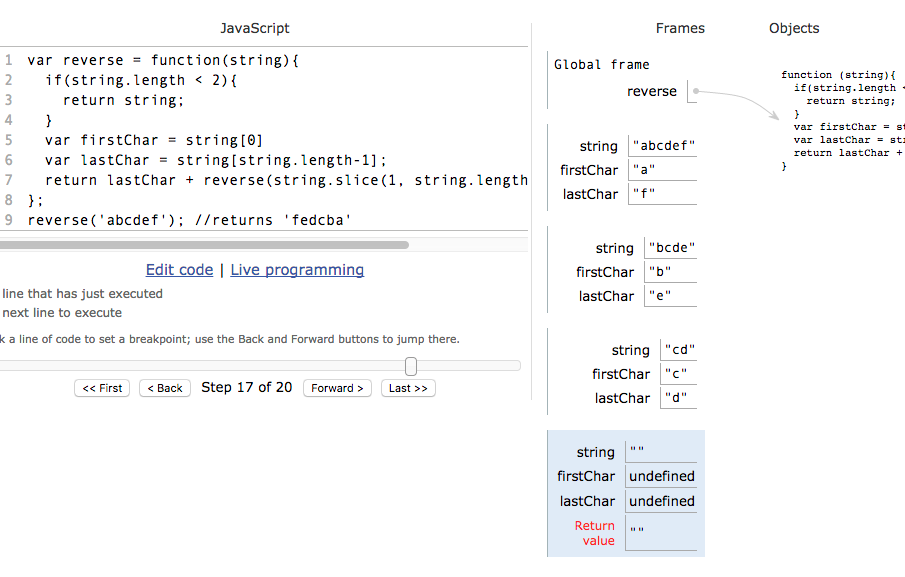
Slow down and follow the interpreter through its execution of your algorithm (thanks to PythonTutor.com)
Python Tutor is an excellent resource for learning to visualize and trace variable values through the multiple execution contexts of a recursive function's invocation.
Try it now with these simple steps:
- copy the solution code from above
- go over to http://pythontutor.com/javascript.html#mode=edit
- paste the solution code into the editor
- click the "Visualize Execution" button
- progress through the execution with the "forward" button
//when can a recursive function help me?
So if I hope that at this point that you are thinking: there is a better way to reverse a function, or there is a simpler way to reverse a string…
First off… simpler is better. Writing good code isn't about being clever or fancy; good code is about writing code that works, that makes sense to as many other minds as possible, that is time efficient, and that is memory efficient (in order of importance). As new programers, the first of these criteria is obvious, and the last two are given way too much weight. It's the second of these criteria that needs to carry much more weight in our minds and deserves the most attention. Recursive functions can be a powerful tool in helping us write clear and simple solutions.
To be clear: recursion is not about being fancy or clever… it is an important skill to wrestle with early because there will be many scenarios when employing recursion will allow for a simpler and more reliable solution than would be possible without recursive functions.
//more useful example
Prompt: check to see if a binary-search-tree contains a value
var searchBST = function(tree, num){
if(tree.val === num){
return true
} else if(num > tree.val){
if(tree.right === null){
     return false;
     } else{
     return searchBST(tree.right, num);
     }
} else{
if(tree.left === null){
     return false;
     } else{
     return searchBST(tree.left, num);
     }
}
}; var tree = {val: 9,
 left: {val: 5,
     left: null,
     right: {val: 7,
     left: null,
     right: null}
     },
     right: {val: 20,
     left: {val: 16,
     left: null,
     right: {val: 18,
     left: null,
     right: null}
     },
     right: null}
     };searchBST(tree, 18) // return true
searchBST(tree, 4) // return false
When traversing trees and many other other non-primative data structures, recursion allows us to define a clear algorithm that elegantly handles uncertainty and complexity. Without recursion, it would be impossible to write a single function that could search a binary search tree of any size and state… yet by employing recursion, we can write a concise algorithm that will traverse any binary search tree and determine if it contains a value or not.
Take a moment to analyze how recursion is used in this example by tracing the interpreters path through this solution. Just as we did for the reverse function above, paste this binary search tree code snippet into the editor at http://pythontutor.com/javascript.html#mode=display
In this function definition, there are three base cases that will return a value instead of recursively calling the searchBST function… can you find them?
//now go practice using recursion
Data Structures and
Algorithms
Big O Memoization And Tabulation - Recursion Videos - Curating Complexity: A Guide to Big-O Notation - Why Big-O? - Big-O Notation - Common Complexity Classes - The seven major classes - Memoization - Memoizing factorial - Memoizing the Fibonacci generator - The memoization formula - Tabulation - Tabulating the Fibonacci number - Aside: Refactoring for O(1) Space - Analysis of Linear Search - Analysis of Binary Search - Analysis of the Merge Sort - Analysis of Bubble Sort - LeetCode.com - Memoization Problems - Tabulation Problems
Sorting Algorithms - Bubble Sort - "But…then…why are we…" - The algorithm bubbles up - How does a pass of Bubble Sort work? - Ending the Bubble Sort - Pseudocode for Bubble Sort - Selection Sort - The algorithm: select the next smallest - The pseudocode - Insertion Sort - The algorithm: insert into the sorted region - The Steps - The pseudocode - Merge Sort - The algorithm: divide and conquer - Quick Sort - How does it work? - The algorithm: divide and conquer - The pseudocode - Binary Search - The Algorithm: "check the middle and half the search space" - The pseudocode - Bubble Sort Analysis - Time Complexity: O(n2) - Space Complexity: O(1) - When should you use Bubble Sort? - Selection Sort Analysis - Selection Sort JS Implementation - Time Complexity Analysis - Space Complexity Analysis: O(1) - When should we use Selection Sort? - Insertion Sort Analysis - Time and Space Complexity Analysis - When should you use Insertion Sort? - Merge Sort Analysis - Full code - Merging two sorted arrays - Divide and conquer, step-by-step - Time and Space Complexity Analysis - Quick Sort Analysis - Time and Space Complexity Analysis - Binary Search Analysis - Time and Space Complexity Analysis - Practice: Bubble Sort - Practice: Selection Sort - Practice: Insertion Sort - Practice: Merge Sort - Practice: Quick Sort - Practice: Binary Search
Lists, Stacks, and Queues - Linked Lists - What is a Linked List? - Types of Linked Lists - Linked List
Methods - Time and Space Complexity Analysis -
Time Complexity - Access and Search - Time Complexity - Insertion and Deletion - Space Complexity - Stacks and Queues -
What is a Stack? - What is a Queue? - Stack and Queue Properties - Stack
Methods - Queue Methods - Time
and Space Complexity Analysis - When should we use Stacks
and Queues? - Graphs and Heaps - Introduction to Heaps - Binary
Heap
Implementation - Heap Sort - In-Place
Heap
Sort - The objective of this lesson is get you comfortable with identifying the time and
space
complexity of code you see. Being able to diagnose time complexity for algorithms is an essential
for
interviewing software engineers. At the end of this, you will be able to At the end of this, you will be able to The objective of this lesson is to give you a couple of ways to optimize a
computation
(algorithm) from a higher complexity class to a lower complexity class. Being able to optimize
algorithms is
an
essential for interviewing software engineers. At the end of this, you will be able to At the end of this, you will be able to A lot of algorithms that we use in the upcoming days will use recursion. The next two videos are just
helpful
reminders about recursion so that you can get that thought process back into your brain. Colt Steele provides a very nice, non-mathy introduction to Big-O notation. Please watch this so you
can get
the
easy introduction. Big-O is, by its very nature, math based. It's good to get an understanding
before
jumping in
to math expressions. Complete Beginner's Guide to Big O Notation
by Colt
Steele. As software engineers, our goal is not just to solve problems. Rather, our goal is to solve problems
efficiently
and elegantly. Not all solutions are made equal! In this section we'll explore how to analyze the
efficiency
of
algorithms in terms of their speed (time complexity) and memory consumption (space
complexity). In this article, we'll use the word efficiency to describe the amount of resources a
program
needs
to execute. The two resources we are concerned with are time and space. Our
goal is to
minimize the amount of time and space that our programs use.
When you finish this article you will be able to: Let's begin by understanding what method we should not use when describing the efficiency of
our
algorithms. Most importantly, we'll want to avoid using absolute units of time when describing
speed. When
the
software engineer exclaims, "My function runs in 0.2 seconds, it's so fast!!!", the computer
scientist is
not
impressed. Skeptical, the computer scientist asks the following questions: The job of the software engineer is to focus on the software detail and not necessarily the hardware
it will
run
on. Because we can't answer points 1 and 2 with total certainty, we'll want to avoid using concrete
units
like
"milliseconds" or "seconds" when describing the efficiency of our algorithms. Instead, we'll opt for
a more
abstract approach that focuses on point 3. This means that we should focus on how the performance of
our
algorithm is affected by increasing the size of the input. In other words, how does our
performance
scale? The argument above focuses on time, but a similar argument could also be made for
space.
For example, we should not analyze our code in terms of the amount of absolute kilobytes of
memory it
uses,
because this is dependent on the programming language.
In Computer Science, we use Big-O notation as a tool for describing the efficiency of algorithms with
respect
to
the size of the input argument(s). We use mathematical functions in Big-O notation, so there are a
few big
picture ideas that we'll want to keep in mind: The first 3 points are conceptual, so they are easy to swallow. However, point 4 is typically the
biggest
source
of confusion when learning the notation. Before we apply Big-O to our code, we'll need to first
understand
the
underlying math and simplification process. We want our Big-O notation to describe the performance of our algorithm with respect to the input
size and
nothing else. Because of this, we should to simplify our Big-O functions using the following rules:
We'll look at these rules in action, but first we'll define a few things: If a function consists of a product of many factors, we drop the factors that don't depend on the
size of the
input, n. The factors that we drop are called constant factors because their size remains consistent
as we
increase the size of the input. The reasoning behind this simplification is that we make the input
large
enough,
the non-constant factors will overshadow the constant ones. Below are some examples:
Big O
Memoization And Tabulation
Recursion Videos
Big-O By Colt Steele
Curating Complexity: A Guide to Big-O Notation
Why Big-O?
Big-O Notation
Simplifying Math Terms
Simplifying a Product
| Unsimplified | Big-O Simplified |
|---|---|
| T( 5 * n2 ) | O( n2 ) |
| T( 100000 * n ) | O( n ) |
| T( n / 12 ) | O( n ) |
| T( 42 * n * log(n) ) | O( n * log(n) ) |
| T( 12 ) | O( 1 ) |
Note that in the third example, we can simplify T( n /
12 ) to O( n
)
because we
can
rewrite a division into an equivalent multiplication. In other words, T( n / 12 ) = T( 1/12 *
n ) = O(
n
).
Simplifying a Sum
If the function consists of a sum of many terms, we only need to show the term that grows the fastest, relative to the size of the input. The reasoning behind this simplification is that if we make the input large enough, the fastest growing term will overshadow the other, smaller terms. To understand which term to keep, you'll need to recall the relative size of our common math terms from the previous section. Below are some examples:
| Unsimplified | Big-O Simplified |
|---|---|
| T( n3 + n2 + n ) | O( n3 ) |
| T( log(n) + 2n ) | O( 2n ) |
| T( n + log(n) ) | O( n ) |
| T( n! + 10n ) | O( n! ) |
Putting it all together
The product and sum rules are all we'll need to Big-O simplify any math functions. We just apply the product rule to drop all constants, then apply the sum rule to select the single most dominant term.
| Unsimplified | Big-O Simplified |
|---|---|
| T( 5n2 + 99n ) | O( n2 ) |
| T( 2n + nlog(n) ) | O( nlog(n) ) |
| T( 2n + 5n1000) | O( 2n ) |
Aside: We'll often omit the multiplication symbol in expressions as a form of shorthand. For example, we'll write O( 5n2 ) in place of O( 5 * n2 ).
RECAP
- explained why Big-O is the preferred notation used to describe the efficiency of algorithms
- used the product and sum rules to simplify mathematical functions into Big-O notation
Common Complexity Classes
Analyzing the efficiency of our code seems like a daunting task because there are many different possibilities in how we may choose to implement something. Luckily, most code we write can be categorized into one of a handful of common complexity classes. In this reading, we'll identify the common classes and explore some of the code characteristics that will lead to these classes.
When you finish this reading, you should be able to:
- name and order the seven common complexity classes
- identify the time complexity class of a given code snippet
The seven major classes
There are seven complexity classes that we will encounter most often. Below is a list of each complexity class as well as its Big-O notation. This list is ordered from smallest to largest. Bear in mind that a "more efficient" algorithm is one with a smaller complexity class, because it requires fewer resources.
| Big-O | Complexity Class Name |
|---|---|
| O(1) | constant |
| O(log(n)) | logarithmic |
| O(n) | linear |
| O(n * log(n)) | loglinear, linearithmic, quasilinear |
| O(nc) - O(n2), O(n3), etc. | polynomial |
| O(cn) - O(2n), O(3n), etc. | exponential |
| O(n!) | factorial |
There are more complexity classes that exist, but these are most common. Let's take a closer look at each of these classes to gain some intuition on what behavior their functions define. We'll explore famous algorithms that correspond to these classes further in the course.
For simplicity, we'll provide small, generic code examples that illustrate the complexity, although they may not solve a practical problem.
O(1) - Constant
Constant complexity means that the algorithm takes roughly the same number of steps for any size input. In a constant time algorithm, there is no relationship between the size of the input and the number of steps required. For example, this means performing the algorithm on a input of size 1 takes the same number of steps as performing it on an input of size 128.
Constant growth
The table below shows the growing behavior of a constant function. Notice that the behavior stays constant for all values of n.
| n | O(1) |
|---|---|
| 1 | ~1 |
| 2 | ~1 |
| 3 | ~1 |
| … | … |
| 128 | ~1 |
Example Constant code
Below is are two examples of functions that have constant runtimes.
// O(1)
function constant1(n) {
  return n * 2 + 1;
}

// O(1)
function constant2(n) {
  for (let i = 1; i <= 100; i++) {
    console.log(i);
  }
}
The runtime of the constant1 function
does not depend on the size of the input, because
only two
arithmetic operations (multiplication and addition) are always performed. The runtime of the
constant2 function also does not
depend on the size of the input because one-hundred
iterations
are
always performed, irrespective of the input.
O(log(n)) - Logarithmic
Typically, the hidden base of O(log(n)) is 2, meaning O(log2(n)). Logarithmic complexity algorithms will usual display a sense of continually "halving" the size of the input. Another tell of a logarithmic algorithm is that we don't have to access every element of the input. O(log2(n)) means that every time we double the size of the input, we only require one additional step. Overall, this means that a large increase of input size will increase the number of steps required by a small amount.
Logarithmic growth
The table below shows the growing behavior of a logarithmic runtime function. Notice that doubling the input size will only require only one additional "step".
| n | O(log2(n)) |
|---|---|
| 2 | ~1 |
| 4 | ~2 |
| 8 | ~3 |
| 16 | ~4 |
| … | … |
| 128 | ~7 |
Example logarithmic code
Below is an example of two functions with logarithmic runtimes.
// O(log(n))
function logarithmic1(n) {
  if (n <= 1) return;
  logarithmic1(n / 2);
}

// O(log(n))
function logarithmic2(n) {
  let i = n;
  while (i > 1) {
    i /= 2;
  }
}
The logarithmic1 function has
O(log(n)) runtime because the recursion will half the
argument, n,
each time. In other words, if we pass 8 as the original argument, then the recursive chain would be
8 ->
4
-> 2 -> 1. In a similar way, the logarithmic2 function has O(log(n)) runtime
because of
the
number of iterations in the while loop. The while loop depends on the variable i, which
will be
divided in half each iteration.
O(n) - Linear
Linear complexity algorithms will access each item of the input "once" (in the Big-O sense). Algorithms that iterate through the input without nested loops or recurse by reducing the size of the input by "one" each time are typically linear.
Linear growth
The table below shows the growing behavior of a linear runtime function. Notice that a change in input size leads to similar change in the number of steps.
| n | O(n) |
|---|---|
| 1 | ~1 |
| 2 | ~2 |
| 3 | ~3 |
| 4 | ~4 |
| … | … |
| 128 | ~128 |
Example linear code
Below are examples of three functions that each have linear runtime.
// O(n)
function linear1(n) {
  for (let i = 1; i <= n; i++) {
    console.log(i);
  }
}

// O(n), where n is the length of the array
function linear2(array) {
  for (let i = 0; i < array.length; i++) {
    console.log(i);
  }
}

// O(n)
function linear3(n) {
  if (n === 1) return;
  linear3(n - 1);
}
The linear1 function has O(n) runtime
because the for loop will iterate n times. The
linear2 function has O(n) runtime
because the for loop iterates through the array
argument. The
linear3 function has O(n) runtime
because each subsequent call in the recursion will
decrease
the
argument by one. In other words, if we pass 8 as the original argument to linear3, the
recursive
chain would be 8 -> 7 -> 6 -> 5 -> … -> 1.
O(n * log(n)) - Loglinear
This class is a combination of both linear and logarithmic behavior, so features from both classes are evident. Algorithms the exhibit this behavior use both recursion and iteration. Typically, this means that the recursive calls will halve the input each time (logarithmic), but iterations are also performed on the input (linear).
Loglinear growth
The table below shows the growing behavior of a loglinear runtime function.
| n | O(n * log2(n)) |
|---|---|
| 2 | ~2 |
| 4 | ~8 |
| 8 | ~24 |
| … | … |
| 128 | ~896 |
Example loglinear code
Below is an example of a function with a loglinear runtime.
// O(n * log(n))
function loglinear(n) {
  if (n <= 1) return;

  for (let i = 1; i <= n; i++) {
    console.log(i);
  }

  loglinear(n / 2);
  loglinear(n / 2);
}
The loglinear function has O(n *
log(n)) runtime because the for loop iterates linearly
(n)
through
the input and the recursive chain behaves logarithmically (log(n)).
O(nc) - Polynomial
Polynomial complexity refers to complexity of the form O(nc) where n is the
size of
the
input and c is some fixed constant.
For example, O(n3) is a larger/worse
function
than
O(n2), but they belong to the same complexity class. Nested loops are usually the
indicator of
this
complexity class.
Polynomial growth
Below are tables showing the growth for O(n2) and O(n3).
| n | O(n2) |
|---|---|
| 1 | ~1 |
| 2 | ~4 |
| 3 | ~9 |
| … | … |
| 128 | ~16,384 |
| n | O(n3) |
|---|---|
| 1 | ~1 |
| 2 | ~8 |
| 3 | ~27 |
| … | … |
| 128 | ~2,097,152 |
Example polynomial code
Below are examples of two functions with polynomial runtimes.
// O(n^2)
function quadratic(n) {
  for (let i = 1; i <= n; i++) {
    for (let j = 1; j <= n; j++) {}
  }
}

// O(n^3)
function cubic(n) {
  for (let i = 1; i <= n; i++) {
    for (let j = 1; j <= n; j++) {
      for (let k = 1; k <= n; k++) {}
    }
  }
}
The quadratic function has
O(n2) runtime because there are nested loops. The
outer
loop
iterates n times and the inner loop iterates n times. This leads to n * n total number of
iterations. In a
similar way, the cubic function has
O(n3) runtime because it has triply
nested loops
that lead to a total of n * n * n iterations.
O(cn) - Exponential
Exponential complexity refers to Big-O functions of the form O(cn) where n is
the
size of
the input and c is some fixed
constant. For example, O(3n) is a larger/worse
function
than O(2n), but they both belong to the exponential complexity class. A common indicator
of this
complexity class is recursive code where there is a constant number of recursive calls in each stack
frame.
The
c will be the number of recursive
calls made in each stack frame. Algorithms with this
complexity
are considered quite slow.
Exponential growth
Below are tables showing the growth for O(2n) and O(3n). Notice how these grow large, quickly.
| n | O(2n) |
|---|---|
| 1 | ~2 |
| 2 | ~4 |
| 3 | ~8 |
| 4 | ~16 |
| … | … |
| 128 | ~3.4028 * 1038 |
| n | O(3n) |
|---|---|
| 1 | ~3 |
| 2 | ~9 |
| 3 | ~27 |
| 3 | ~81 |
| … | … |
| 128 | ~1.1790 * 1061 |
Exponential code example
Below are examples of two functions with exponential runtimes.
// O(2^n)
function exponential2n(n) {
  if (n === 1) return;
  exponential_2n(n - 1);
  exponential_2n(n - 1);
}

// O(3^n)
function exponential3n(n) {
  if (n === 0) return;
  exponential_3n(n - 1);
  exponential_3n(n - 1);
  exponential_3n(n - 1);
}
The exponential2n function has
O(2n) runtime because each call will make two
more
recursive calls. The exponential3n
function has O(3n) runtime because each
call will
make three more recursive calls.
O(n!) - Factorial
Recall that n! = (n) * (n - 1) * (n - 2) *
... * 1. This complexity is typically the
largest/worst
that we will end up implementing. An indicator of this complexity class is recursive code that has a
variable
number of recursive calls in each stack frame. Note that factorial is worse than
exponential
because factorial algorithms have a variable amount of recursive calls in each
stack
frame,
whereas exponential algorithms have a constant amount of recursive calls in each
frame.
Factorial growth
Below is a table showing the growth for O(n!). Notice how this has a more aggressive growth than exponential behavior.
| n | O(n!) |
|---|---|
| 1 | ~1 |
| 2 | ~2 |
| 3 | ~6 |
| 4 | ~24 |
| … | … |
| 128 | ~3.8562 * 10215 |
Factorial code example
Below is an example of a function with factorial runtime.
// O(n!)
function factorial(n) {
  if (n === 1) return;

  for (let i = 1; i <= n; i++) {
    factorial(n - 1);
  }
}
The factorial function has O(n!)
runtime because the code is recursive but the
number
of
recursive calls made in a single stack frame depends on the input. This contrasts with an
exponential
function because exponential functions have a fixed number of calls in each stack frame.
You may it difficult to identify the complexity class of a given code snippet, especially if the code falls into the loglinear, exponential, or factorial classes. In the upcoming videos, we'll explain the analysis of these functions in greater detail. For now, you should focus on the relative order of these seven complexity classes!
RECAP
In this reading, we listed the seven common complexity classes and saw some example code for each. In order of ascending growth, the seven classes are:
- Constant
- Logarithmic
- Linear
- Loglinear
- Polynomial
- Exponential
- Factorial
Self-Similarity
Recursion is the root of computation since it trades description for time.—Alan Perlis, Epigrams in Programming
In Arrays and Destructuring Arguments, we worked with the basic idea that putting an array together with a literal array expression was the reverse or opposite of taking it apart with a destructuring assignment.
We saw that the basic idea that putting an array together with a literal array expression was the reverse or opposite of taking it apart with a destructuring assignment.
Let's be more specific. Some data structures, like lists, can obviously be seen as a collection of items. Some are empty, some have three items, some forty-two, some contain numbers, some contain strings, some a mixture of elements, there are all kinds of lists.
But we can also define a list by describing a rule for building lists. One of the simplest, and longest-standing in computer science, is to say that a list is:
- Empty, or;
- Consists of an element concatenated with a list .
Let's convert our rules to array literals. The first rule is simple: []
is a list. How about the
second rule? We can express that using a spread. Given an element e and
a list list ,
[e, ...list] is a list. We can test this manually by
building up a
list:
[]
                      //=> []

                      ["baz", ...[]]
                      //=> ["baz"]

                      ["bar", ...["baz"]]
                      //=> ["bar","baz"]

                      ["foo", ...["bar", "baz"]]
                      //=> ["foo","bar","baz"]
Thanks to the parallel between array literals + spreads with destructuring + rests, we can also use the same rules to decompose lists:
const [first, ...rest] = [];
                      first
                      //=> undefined
                      rest
                      //=> []:

                      const [first, ...rest] = ["foo"];
                      first
                      //=> "foo"
                      rest
                      //=> []

                      const [first, ...rest] = ["foo", "bar"];
                      first
                      //=> "foo"
                      rest
                      //=> ["bar"]

                      const [first, ...rest] = ["foo", "bar", "baz"];
                      first
                      //=> "foo"
                      rest
                      //=> ["bar","baz"]
For the purpose of this exploration, we will presume the following:1
const isEmpty = ([first, ...rest]) => first === undefined;

                      isEmpty([])
                      //=> true

                      isEmpty([0])
                      //=> false

                      isEmpty([[]])
                      //=> false
Armed with our definition of an empty list and with what we've already learned, we can build a
great many
functions that operate on arrays. We know that we can get the length of an array using its .length
. But as an exercise, how would we write a length
function using just
what we have already?
First, we pick what we call a terminal case. What is the length of an empty array? 0 . So
let's start our function with the observation that if an array is empty, the length is 0 :
const length = ([first, ...rest]) =>
                      first === undefined
                      ? 0
                      : // ???
We need something for when the array isn't empty. If an array is not empty, and we break it into
two pieces,
first and rest ,
the length of
our array is going to be length(first) +
length(rest) . Well, the length of first is
1 , there's just one element at
the front. But we don't know the length of rest . If only
there was a
function we could call… Like
length !
const length = ([first, ...rest]) =>
                      first === undefined
                      ? 0
                      : 1 + length(rest);
Let's try it!
length([])
                      //=> 0


                      length(["foo"])
                      //=> 1


                      length(["foo", "bar", "baz"])
                      //=> 3
Our length function is recursive, it calls
itself. This makes
sense because our definition
of a list is recursive, and if a list is self-similar, it is natural to create an algorithm that
is also
self-similar.
linear recursion
"Recursion" sometimes seems like an elaborate party trick. There's even a joke about this:
When promising students are trying to choose between pure mathematics and applied engineering, they are given a two-part aptitude test. In the first part, they are led to a laboratory bench and told to follow the instructions printed on the card. They find a bunsen burner, a sparker, a tap, an empty beaker, a stand, and a card with the instructions "boil water."
Of course, all the students know what to do: They fill the beaker with water, place the stand on the burner and the beaker on the stand, then they turn the burner on and use the sparker to ignite the flame. After a bit the water boils, and they turn off the burner and are lead to a second bench.
Once again, there is a card that reads, "boil water." But this time, the beaker is on the stand over the burner, as left behind by the previous student. The engineers light the burner immediately. Whereas the mathematicians take the beaker off the stand and empty it, thus reducing the situation to a problem they have already solved.
There is more to recursive solutions that simply functions that invoke themselves. Recursive algorithms follow the "divide and conquer" strategy for solving a problem:
- Divide the problem into smaller problems
- If a smaller problem is solvable, solve the small problem
- If a smaller problem is not solvable, divide and conquer that problem
- When all small problems have been solved, compose the solutions into one big solution
The big elements of divide and conquer are a method for decomposing a problem into smaller problems, a test for the smallest possible problem, and a means of putting the pieces back together. Our solutions are a little simpler in that we don't really break a problem down into multiple pieces, we break a piece off the problem that may or may not be solvable, and solve that before sticking it onto a solution for the rest of the problem.
This simpler form of "divide and conquer" is called linear recursion. It's very useful and simple to understand. Let's take another example. Sometimes we want to flatten an array, that is, an array of arrays needs to be turned into one array of elements that aren't arrays.2
We already know how to divide arrays into smaller pieces. How do we decide whether a smaller problem is solvable? We need a test for the terminal case. Happily, there is something along these lines provided for us:
Array.isArray("foo")
                      //=> false

                      Array.isArray(["foo"])
                      //=> true
The usual "terminal case" will be that flattening an empty array will produce an empty array. The next terminal case is that if an element isn't an array, we don't flatten it, and can put it together with the rest of our solution directly. Whereas if an element is an array, we'll flatten it and put it together with the rest of our solution.
So our first cut at a flatten function will look like
this:
const flatten = ([first, ...rest]) => {
                      if (first === undefined) {
                      return [];
                      }
                      else if (! Array.isArray(first)) {
                      return [first, ...flatten(rest)];
                      }
                      else {
                      return [...flatten(first), ...flatten(rest)];
                      }
                      }


                      flatten(["foo", [3, 4, []]])
                      //=> ["foo", 3, 4]
Once again, the solution directly displays the important elements: Dividing a problem into subproblems, detecting terminal cases, solving the terminal cases, and composing a solution from the solved portions.
mapping
Another common problem is applying a function to every element of an array. JavaScript has a built-in function for this, but let's write our own using linear recursion.
If we want to square each number in a list, we could write:
const squareAll = ([first, ...rest]) => first === undefined
                      ? []
                      : [first * first, ...squareAll(rest)];

                      squareAll([1, 2, 3, 4, 5])
                      //=> [1,4,9,16,25]
And if we wanted to "truthify" each element in a list, we could write:
const truthyAll = ([first, ...rest]) => first === undefined
                      ? []
                      : [!!first, ...truthyAll(rest)];

                      truthyAll([null, true, 25, false, "foo"])
                      //=> [false,true,true,false,true]
This specific case of linear recursion is called "mapping," and it is not necessary to constantly write out the same pattern again and again. Functions can take functions as arguments, so let's "extract" the thing to do to each element and separate it from the business of taking an array apart, doing the thing, and putting the array back together.
Given the signature:
const mapWith = (fn, array) => // ...
We can write it out using a ternary operator. Even in this small function, we can identify the terminal condition, the piece being broken off, and recomposing the solution.
const mapWith = (fn, [first, ...rest]) =>
                      first === undefined
                      ? []
                      : [fn(first), ...mapWith(fn, rest)];

                      mapWith((x) => x * x, [1, 2, 3, 4, 5])
                      //=> [1,4,9,16,25]

                      mapWith((x) => !!x, [null, true, 25, false, "foo"])
                      //=> [false,true,true,false,true]
folding
With the exception of the length example at the beginning,
our examples
so far all involve
rebuilding a solution using spreads. But they needn't. A function to compute the sum of the
squares of a list of
numbers might look like this:
const sumSquares = ([first, ...rest]) => first === undefined
                      ? 0
                      : first * first + sumSquares(rest);

                      sumSquares([1, 2, 3, 4, 5])
                      //=> 55
There are two differences between sumSquares and our maps
above:
- Given the terminal case of an empty list, we return a
0instead of an empty list, and; - We catenate the square of each element to the result of applying
sumSquaresto the rest of the elements.
Let's rewrite mapWith so that we can use it to sum
squares.
const foldWith = (fn, terminalValue, [first, ...rest]) =>
                      first === undefined
                      ? terminalValue
                      : fn(first, foldWith(fn, terminalValue, rest));
And now we supply a function that does slightly more than our mapping functions:
foldWith((number, rest) => number * number + rest, 0, [1, 2, 3,
                      4, 5])
                      //=> 55
Our foldWith function is a generalization of our mapWith function. We can represent a
map as a fold, we just need to supply the array rebuilding code:
const squareAll = (array) => foldWith((first, rest) => [first
                      * first,
                      ...rest], [], array);


                      squareAll([1, 2, 3, 4, 5])
                      //=> [1, 4, 9, 16, 25]
And if we like, we can write mapWith using foldWith :
const mapWith = (fn, array) => foldWith((first, rest) =>
                      [fn(first),
                      ...rest], [], array),
                      squareAll = (array) => mapWith((x) => x * x, array);


                      squareAll([1, 2, 3, 4, 5])
                      //=> [1, 4, 9, 16, 25]
And to return to our first example, our version of length
can be written
as a fold:
const length = (array) => foldWith((first, rest) => 1 + rest,
                      0, array);


                      length([1, 2, 3, 4, 5])
                      //=> 5
summary
Linear recursion is a basic building block of algorithms. Its basic form parallels the way linear data structures like lists are constructed: This helps make it understandable. Its specialized cases of mapping and folding are especially useful and can be used to build other functions. And finally, while folding is a special case of linear recursion, mapping is a special case of folding.
-
Well, actually, this does not work for arrays that contain
undefinedas a value, but we are not going to see that in our examples. A more robust implementation would be(array) => array.length === 0, but we are doing backflips to keep this within a very small and contrived playground.↩ -
flattenis a very simple unfold, a function that takes a seed value and turns it into an array. Unfolds can be thought of a "path" through a data structure, and flattening a tree is equivalent to a depth-first traverse.↩
Memoization
Memoization is a design pattern used to reduce the overall number of calculations that can occur in algorithms that use recursive strategies to solve.
Recall that recursion solves a large problem by dividing it into smaller sub-problems that are more manageable. Memoization will store the results of the sub-problems in some other data structure, meaning that you avoid duplicate calculations and only "solve" each subproblem once. There are two features that comprise memoization:
- the function is recursive
- the additional data structure used is typically an object (we refer to this as the memo!)
This is a trade-off between the time it takes to run an algorithm (without memoization) and the memory used to run the algorithm (with memoization). Usually memoization is a good trade-off when dealing with large data or calculations.
You cannot always apply this technique to recursive problems. The problem must have an "overlapping subproblem structure" for memoization to be effective.
Here's an example of a problem that has such a structure:
Using pennies, nickels, dimes, and quarters, what is the smallest combination of coins that total 27 cents?
You'll explore this exact problem in depth later on. For now, here is some food for thought. Along the way to calculating the smallest coin combination of 27 cents, you should also calculate the smallest coin combination of say, 25 cents as a component of that problem. This is the essence of an overlapping subproblem structure.
Memoizing factorial
Here's an example of a function that computes the factorial of the number passed into it.
function factorial(n) {
  if (n === 1) return 1;
  return n * factorial(n - 1);
}

factorial(6);       // => 720, requires 6 calls
factorial(6);       // => 720, requires 6 calls
factorial(5);       // => 120, requires 5 calls
factorial(7);       // => 5040, requires 7 calls
From this plain factorial above, it
is clear that every time you call
factorial(6)
you
should get the same result of 720
each time. The code is somewhat inefficient because
you must
go
down the full recursive stack for each top level call to factorial(6). It would be
great if you
could store the result of factorial(6) the first
time you calculate it, then on
subsequent
calls to
factorial(6) you simply fetch the
stored result in constant time. You can accomplish
exactly
this
by memoizing with an object!
let memo = {}

function factorial(n) {
  // if this function has calculated factorial(n) previously,
  // fetch the stored result in memo
  if (n in memo) return memo[n];
  if (n === 1) return 1;

  // otherwise, it havs not calculated factorial(n) previously,
  // so calculate it now, but store the result in case it is
  // needed again in the future
  memo[n] = n * factorial(n - 1);
  return memo[n]
}

factorial(6);       // => 720, requires 6 calls
factorial(6);       // => 720, requires 1 call
factorial(5);       // => 120, requires 1 call
factorial(7);       // => 5040, requires 2 calls

memo;   // => { '2': 2, '3': 6, '4': 24, '5': 120, '6': 720, '7': 5040 }
The memo object above will map an
argument of factorial to its return
value. That
is,
the keys will be arguments and their values will be the corresponding results returned. By using the
memo,
you
are able to avoid duplicate recursive calls!
Here's some food for thought: By the time your first call to factorial(6) returns, you
will not
have
just the argument 6 stored in the
memo. Rather, you will have all arguments 2
to 6
stored
in the memo.
Hopefully you sense the efficiency you can get by memoizing your functions, but maybe you are not convinced by the last example for two reasons:
- You didn't improve the speed of the algorithm by an order of Big-O (it is still O(n)).
- The code uses some global variable, so it's kind of ugly.
Both of those points are true, so take a look at a more advanced example that benefits from memoization.
Memoizing the Fibonacci generator
Here's a naive implementation of a function that calculates the Fibonacci number for a given input.
function fib(n) {
  if (n === 1 || n === 2) return 1;
  return fib(n - 1) + fib(n - 2);
}

fib(6);     // => 8
Before you optimize this, ask yourself what complexity class it falls into in the first place.
The time complexity of this function is not super intuitive to describe because the code branches twice recursively. Fret not! You'll find it useful to visualize the calls needed to do this with a tree. When reasoning about the time complexity for recursive functions, draw a tree that helps you see the calls. Every node of the tree represents a call of the recursion:

In general, the height of this tree will be n.
You derive this by following the path
going
straight
down the left side of the tree. You can also see that each internal node leads to two more nodes.
Overall,
this
means that the tree will have roughly 2n nodes which is the same as saying that the
fib
function has an exponential time complexity of 2n. That is very slow! See for yourself,
try
running
fib(50) - you'll be waiting for
quite a while (it took 3 minutes on the author's
machine).
Okay. So the fib function is slow. Is
there anyway to speed it up? Take a look at the
tree
above.
Can you find any repetitive regions of the tree?

As the n grows bigger, the number of
duplicate sub-trees grows exponentially. Luckily
you can
fix
this using memoization by using a similar object strategy as before. You can use some JavaScript
default
arguments to clean things up:
function fastFib(n, memo = {}) {
  if (n in memo) return memo[n];
  if (n === 1 || n === 2) return 1;

  memo[n] = fastFib(n - 1, memo) + fastFib(n - 2, memo);
  return memo[n];
}

fastFib(6);     // => 8
fastFib(50);    // => 12586269025
The code above can calculate the 50th Fibonacci number almost instantly! Thanks to the
memo
object,
you only need to explore a subtree fully once. Visually, the fastFib recursion has this
structure:

You can see the marked nodes (function calls) that access the memo in green. It's easy to see that
this
version
of the Fibonacci generator will do far less computations as n grows larger! In fact,
this
memoization has brought the time complexity down to linear O(n) time because the tree
only
branches
on the left side. This is an enormous gain if you recall the complexity class hierarchy.
The memoization formula
Now that you understand memoization, when should you apply it? Memoization is useful when attacking recursive problems that have many overlapping sub-problems. You'll find it most useful to draw out the visual tree first. If you notice duplicate sub-trees, time to memoize. Here are the hard and fast rules you can use to memoize a slow function:
- Write the unoptimized, brute force recursion and make sure it works.
- Add the memo object as an additional argument to the function. The keys will represent unique arguments to the function, and their values will represent the results for those arguments.
- Add a base case condition to the function that returns the stored value if the function's argument is in the memo.
- Before you return the result of the recursive case, store it in the memo as a value and make the function's argument it's key.
What you learned
You learned a secret to possibly changing an algorithm of one complexity class to a lower complexity class by using memory to store intermediate results. This is a powerful technique to use to make sure your programs that must do recursive calculations can benefit from running much faster.
Tabulation
Now that you are familiar with memoization, you can explore a related method of algorithmic optimization: Tabulation. There are two main features that comprise the Tabulation strategy:
- the function is iterative and not recursive
- the additional data structure used is typically an array, commonly referred to as the table
Many problems that can be solved with memoization can also be solved with tabulation as long as you convert the recursion to iteration. The first example is the canonical example of recursion, calculating the Fibonacci number for an input. However, in the example, you'll see the iteration version of it for a fresh start!
Tabulating the Fibonacci number
Tabulation is all about creating a table (array) and filling it out with elements. In general, you will complete the table by filling entries from "left to right". This means that the first entry of the table (first element of the array) will correspond to the smallest subproblem. Naturally, the final entry of the table (last element of the array) will correspond to the largest problem, which is also the final answer.
Here's a way to use tabulation to store the intermediary calculations so that later calculations can refer back to the table.
function tabulatedFib(n) {
  // create a blank array with n reserved spots
  let table = new Array(n);

  // seed the first two values
  table[0] = 0;
  table[1] = 1;

  // complete the table by moving from left to right,
  // following the fibonacci pattern
  for (let i = 2; i <= n; i += 1) {
    table[i] = table[i - 1] + table[i - 2];
  }

  return table[n];
}

console.log(tabulatedFib(7));      // => 13
When you initialized the table and seeded the first two values, it looked like this:
| i | 0 | 1 | 2 | 3 | 4 | 5 | 6 | 7 |
|---|---|---|---|---|---|---|---|---|
table[i] |
0 |
1 |
After the loop finishes, the final table will be:
| i | 0 | 1 | 2 | 3 | 4 | 5 | 6 | 7 |
|---|---|---|---|---|---|---|---|---|
table[i] |
0 |
1 |
1 |
2 |
3 |
5 |
8 |
13 |
Similar to the previous memo, by the
time the function completes, the table
will
contain the final solution as well as all sub-solutions calculated along the way.
To compute the complexity class of this tabulatedFib is very straightforward since the
code is
iterative. The dominant operation in the function is the loop used to fill out the entire table. The
length
of
the table is roughly n elements
long, so the algorithm will have an O(n)
runtime. The
space taken by our algorithm is also O(n) due to the size of the table. Overall, this
should be a
satisfying solution for the efficiency of the algorithm.
Aside: Refactoring for O(1) Space
You may notice that you can cut down on the space used by the function. At any point of the loop, the calculation really only need the previous two subproblems' results. There is little utility to storing the full array. This refactor is easy to do by using two variables:
function fib(n) {
  let mostRecentCalcs = [0, 1];

  if (n === 0) return mostRecentCalcs[0];

  for (let i = 2; i <= n; i++) {
    const [ secondLast, last ] = mostRecentCalcs;
    mostRecentCalcs = [ last, secondLast + last ];
  }

  return mostRecentCalcs[1];
}
Bam! You now have O(n) runtime and O(1) space. This is the most optimal algorithm for calculating a Fibonacci number. Note that this strategy is a pared down form of tabulation, since it uses only the last two values.
The Tabulation Formula
Here are the general guidelines for implementing the tabulation strategy. This is just a general recipe, so adjust for taste depending on your problem:
- Create the table array based off of the size of the input, which isn't always straightforward if you have multiple input values
- Initialize some values in the table that "answer" the trivially small subproblem usually by initializing the first entry (or entries) of the table
- Iterate through the array and fill in remaining entries, using previous entries in the table to perform the current calculation
- Your final answer is (usually) the last entry in the table
What you learned
You learned another way of possibly changing an algorithm of one complexity class to a lower complexity class by using memory to store intermediate results. This is a powerful technique to use to make sure your programs that must do iterative calculations can benefit from running much faster.
Analysis of Linear Search
Consider the following search algorithm known as linear search.
function search(array, term) {
  for (let i = 0; i < array.length; i++) {
    if (array[i] == term) {
      return i;
    }
  }
  return -1;
}
Most Big-O analysis is done on the "worst-case scenario" and provides an upper bound. In the worst case analysis, you calculate the upper bound on running time of an algorithm. You must know the case that causes the maximum number of operations to be executed.
For linear search, the worst case happens when the element to be searched (term
in the
above code) is not present in the array. When term
is not present, the
search
function
compares it with all the elements of array one by
one. Therefore, the worst-case time
complexity of
linear search would be O(n).
Analysis of Binary Search
Consider the following search algorithm known as the binary search. This kind of search only works if the array is already sorted.
function binarySearch(arr, x, start, end) {
  if (start > end) return false;

  let mid = Math.floor((start + end) / 2);
  if (arr[mid] === x) return true;

  if (arr[mid] > x) {
    return binarySearch(arr, x, start, mid - 1);
  } else {
    return binarySearch(arr, x, mid + 1, end);
  }
}
For the binary search, you cut the search space in half every time. This means that it reduces the number of searches you must do by half, every time. That means the number of steps it takes to get to the desired item (if it exists in the array), in the worst case takes the same amount of steps for every number within a range defined by the powers of 2.
- 7 -> 4 -> 2 -> 1
- 8 -> 4 -> 2 -> 1
- 9 -> 5 -> 3 -> 2 -> 1
- 15 -> 8 -> 4 -> 2 -> 1
- 16 -> 8 -> 4 -> 2 -> 1
- 17 -> 9 -> 5 -> 3 -> 2 -> 1
- 31 -> 16 -> 8 -> 4 -> 2 -> 1
- 32 -> 16 -> 8 -> 4 -> 2 -> 1
- 33 -> 17 -> 9 -> 5 -> 3 -> 2 -> 1
So, for any number of items in the sorted array between 2n-1 and 2n, it takes n number of steps. That means if you have k items in the array, then it will take log2k.
Binary searches are O(log2n).
Analysis of the Merge Sort
Consider the following divide-and-conquer sort method known as the merge sort.
function merge(leftArray, rightArray) {
  const sorted = [];
  while (leftArray.length > 0 && rightArray.length > 0) {
    const leftItem = leftArray[0];
    const rightItem = rightArray[0];

    if (leftItem > rightItem) {
      sorted.push(rightItem);
      rightArray.shift();
    } else {
      sorted.push(leftItem);
      leftArray.shift();
    }
  }

  while (leftArray.length !== 0) {
    const value = leftArray.shift();
    sorted.push(value);
  }

  while (rightArray.length !== 0) {
    const value = rightArray.shift();
    sorted.push(value);
  }

  return sorted
}

function mergeSort(array) {
  const length = array.length;
  if (length == 1) {
    return array;
  }

  const middleIndex = Math.ceil(length / 2);
  const leftArray = array.slice(0, middleIndex);
  const rightArray = array.slice(middleIndex, length);

  leftArray = mergeSort(leftArray);
  rightArray = mergeSort(rightArray);

  return merge(leftArray, rightArray);
}
For the merge sort, you cut the sort space in half every time. In each of those halves, you have to loop through the number of items in the array. That means that, for the worst case, you get that same log2n but it must be multiplied by the number of elements in the array, n.
Merge sorts are O(n*log2n).
Analysis of Bubble Sort
Consider the following sort algorithm known as the bubble sort.
function bubbleSort(items) {
  var length = items.length;
  for (var i = 0; i < length; i++) {
    for (var j = 0; j < (length - i - 1); j++) {
      if (items[j] > items[j + 1]) {
        var tmp = items[j];
        items[j] = items[j + 1];
        items[j + 1] = tmp;
      }
    }
  }
}
For the bubble sort, the worst case is the same as the best case because it always makes nested loops. So, the outer loop loops the number of times of the items in the array. For each one of those loops, the inner loop loops again a number of times for the items in the array. So, if there are n values in the array, then a loop inside a loop is n * n. So, this is O(n2). That's polynomial, which ain't that good.
LeetCode.com
use the LeetCode platform to check your work rather than relying on local mocha tests. If you don't already have an account at LeetCode.com, please click https://leetcode.com/accounts/signup/ to sign up for a free account.
After you sign up for the account, please verify the account with the email address that you used so that you can actually run your solution on LeetCode.com.
In the projects, you will see files that are named "leet_code_«number».js". When you open those, you will see a link in the file that you can use to go directly to the corresponding problem on LeetCode.com.
Use the local JavaScript file in Visual Studio Code to collaborate on the solution. Then, you can run the proposed solution in the LeetCode.com code runner to validate its correctness.
Memoization Problems
This project contains two test-driven problems and one problem on LeetCode.com.
- Clone the project from https://github.com/appacademy-starters/algorithms-memoization-project.
cdinto the project foldernpm installto install dependencies in the project root directorynpx testto run the specs- You can view the test cases in
/test/test.js. Your job is to write code in the/libfiles to pass all specs.- In
problems.js, you will write code to make thelucasNumberMemoandminChangefunctions pass. - In
leet_code_518.js, you will use that file as a scratch pad to work on the LeetCode.com problem at https://leetcode.com/problems/coin-change-2/.
- In
Tabulation Problems
This project contains two test-driven problems and one problem on LeetCode.com.
- Clone the project from https://github.com/appacademy-starters/algorithms-tabulation-project.
cdinto the project foldernpm installto install dependencies in the project root directorynpx testto run the specs- You can view the test cases in
/test/test.js. Your job is to write code in the/libfiles to pass all specs.- In
problems.js, you will write code to make thestepper,maxNonAdjacentSum, andminChangefunctions pass. - In
leet_code_64.js, you will use that file as a scratch pad to work on the LeetCode.com problem at https://leetcode.com/problems/minimum-path-sum/. - In
leet_code_70.js, you will use that file as a scratch pad to work on the LeetCode.com problem at https://leetcode.com/problems/climbing-stairs/.
- In
WEEK-07 DAY-3
Sorting
Algorithms
Sorting Algorithms
The objective of this lesson is for you to get experience implementing common sorting algorithms that will come up during a lot of interviews. It is also important for you to understand how different sorting algorithms behave when given output.
At the end of this, you will be able to
- Explain the complexity of and write a function that performs
bubble sorton an array of numbers. - Explain the complexity of and write a function that performs
selection sorton an array of numbers. - Explain the complexity of and write a function that performs
insertion sorton an array of numbers. - Explain the complexity of and write a function that performs
merge sorton an array of numbers. - Explain the complexity of and write a function that performs
quick sorton an array of numbers. - Explain the complexity of and write a function that performs a binary search on a sorted array of numbers.nce implementing common sorting algorithms that will come up during a lot of interviews. It is also important for you to understand how different sorting algorithms behave when given output.
At the end of this, you will be able to
- Explain the complexity of and write a function that performs
bubble sorton an array of numbers. - Explain the complexity of and write a function that performs
selection sorton an array of numbers. - Explain the complexity of and write a function that performs
insertion sorton an array of numbers. - Explain the complexity of and write a function that performs
merge sorton an array of numbers. - Explain the complexity of and write a function that performs
quick sorton an array of numbers. - Explain the complexity of and write a function that performs a binary search on a sorted array of numbers.
Bubble Sort
Bubble Sort is generally the first major sorting algorithm to come up in most introductory programming courses. Learning about this algorithm is useful educationally, as it provides a good introduction to the challenges you face when tasked with converting unsorted data into sorted data, such as conducting logical comparisons, making swaps while iterating, and making optimizations. It's also quite simple to implement, and can be done quickly.
Bubble Sort is almost never a good choice in production. simply because:
- It is not efficient
- It is not commonly used
- There is a stigma attached to using it
"But…then…why are we…"
It is quite useful as an educational base for you, and as a conversational base for you while interviewing, because you can discuss how other more elegant and efficient algorithms improve upon it. Taking naive code and improving upon it by weighing the technical tradeoffs of your other options is 100% the name of the game when trying to level yourself up from a junior engineer to a senior engineer.
The algorithm bubbles up
As you progress through the algorithms and data structures of this course, you'll eventually notice that there are some recurring funny terms. "Bubbling up" is one of those terms.
When someone writes that an item in a collection "bubbles up," you should infer that:
- The item is in motion
- The item is moving in some direction
- The item has some final resting destination
When invoking Bubble Sort to sort an array of integers in ascending order, the largest integers will "bubble up" to the "top" (the end) of the array, one at a time.
The largest values are captured, put into motion in the direction defined by the desired sort (ascending right now), and traverse the array until they arrive at their end destination. See if you can observe this behavior in the following animation (courtesy http://visualgo.net):

As the algorithm iterates through the array, it compares each element to the element's right neighbor. If the current element is larger than its neighbor, the algorithm swaps them. This continues until all elements in the array are sorted.
How does a pass of Bubble Sort work?
Bubble sort works by performing multiple passes to move elements closer to their final positions. A single pass will iterate through the entire array once.
A pass works by scanning the array from left to right, two elements at a time, and checking if they are ordered correctly. To be ordered correctly the first element must be less than or equal to the second. If the two elements are not ordered properly, then we swap them to correct their order. Afterwards, it scans the next two numbers and continue repeat this process until we have gone through the entire array.
See one pass of bubble sort on the array [2,
8, 5, 2, 6]. On each step the elements
currently
being
scanned are in bold.
- [2, 8, 5, 2, 6] - ordered, so leave them alone
- [2, 8, 5, 2, 6] - not ordered, so swap
- [2, 5, 8, 2, 6] - not ordered, so swap
- [2, 5, 2, 8, 6] - not ordered, so swap
- [2, 5, 2, 6, 8] - the first pass is complete
Because at least one swap occurred, the algorithm knows that it wasn't sorted. It needs to make another pass. It starts over again at the first entry and goes to the next-to-last entry doing the comparisons, again. It only needs to go to the next-to-last entry because the previous "bubbling" put the largest entry in the last position.
- [2, 5, 2, 6, 8] - ordered, so leave them alone
- [2, 5, 2, 6, 8] - not ordered, so swap
- [2, 2, 5, 6, 8] - ordered, so leave them alone
- [2, 2, 5, 6, 8] - the second pass is complete
Because at least one swap occurred, the algorithm knows that it wasn't sorted. Now, it can bubble from the first position to the last-2 position because the last two values are sorted.
- [2, 2, 5, 6, 8] - ordered, so leave them alone
- [2, 2, 5, 6, 8] - ordered, so leave them alone
- [2, 2, 5, 6, 8] - the third pass is complete
No swap occurred, so the Bubble Sort stops.
Ending the Bubble Sort
During Bubble Sort, you can tell if the array is in sorted order by checking if a swap was made during the previous pass performed. If a swap was not performed during the previous pass, then the array must be totally sorted and the algorithm can stop.
You're probably wondering why that makes sense. Recall that a pass of Bubble Sort checks if any adjacent elements are out of order and swaps them if they are. If we don't make any swaps during a pass, then everything must be already in order, so our job is done. Let that marinate for a bit.
Pseudocode for Bubble Sort
Bubble Sort: (array)
  n := length(array)
  repeat
  swapped = false
  for i := 1 to n - 1 inclusive do

      /* if this pair is out of order */
      if array[i - 1] > array[i] then

        /* swap them and remember something changed */
        swap(array, i - 1, i)
        swapped := true

      end if
    end for
  until not swapped
Selection Sort
Selection Sort is very similar to Bubble Sort. The major difference between the two is that Bubble Sort bubbles the largest elements up to the end of the array, while Selection Sort selects the smallest elements of the array and directly places them at the beginning of the array in sorted position. Selection sort will utilize swapping just as bubble sort did. Let's carefully break this sorting algorithm down.
The algorithm: select the next smallest
Selection sort works by maintaining a sorted region on the left side of the input array; this sorted region will grow by one element with every "pass" of the algorithm. A single "pass" of selection sort will select the next smallest element of unsorted region of the array and move it to the sorted region. Because a single pass of selection sort will move an element of the unsorted region into the sorted region, this means a single pass will shrink the unsorted region by 1 element whilst increasing the sorted region by 1 element. Selection sort is complete when the sorted region spans the entire array and the unsorted region is empty!

The algorithm can be summarized as the following:
- Set MIN to location 0
- Search the minimum element in the list
- Swap with value at location MIN
- Increment MIN to point to next element
- Repeat until list is sorted
The pseudocode
In pseudocode, the Selection Sort can be written as this.
procedure selection sort
   list  : array of items
   n     : size of list

   for i = 1 to n - 1
   /* set current element as minimum*/
      min = i

      /* check the element to be minimum */

      for j = i+1 to n
         if list[j] < list[min] then
            min = j;
         end if
      end for

      /* swap the minimum element with the current element*/
      if indexMin != i  then
         swap list[min] and list[i]
      end if
   end for
end procedure
Insertion Sort
With Bubble Sort and Selection Sort now in your tool box, you're starting to get some experience points under your belt! Time to learn one more "naive" sorting algorithm before you get to the efficient sorting algorithms.
The algorithm: insert into the sorted region
Insertion Sort is similar to Selection Sort in that it gradually builds up a larger and larger sorted region at the left-most end of the array.
However, Insertion Sort differs from Selection Sort because this algorithm does not focus on searching for the right element to place (the next smallest in our Selection Sort) on each pass through the array. Instead, it focuses on sorting each element in the order they appear from left to right, regardless of their value, and inserting them in the most appropriate position in the sorted region.
See if you can observe the behavior described above in the following animation:

The Steps
Insertion Sort grows a sorted array on the left side of the input array by:
- If it is the first element, it is already sorted. return 1;
- Pick next element
- Compare with all elements in the sorted sub-list
- Shift all the elements in the sorted sub-list that is greater than the value to be sorted
- Insert the value
- Repeat until list is sorted
These steps are easy to confuse with selection sort, so you'll want to watch the video lecture and drawing that accompanies this reading as always!
The pseudocode
procedure insertionSort( A : array of items )
   int holePosition
   int valueToInsert

   for i = 1 to length(A) inclusive do:

      /* select value to be inserted */
      valueToInsert = A[i]
      holePosition = i

      /*locate hole position for the element to be inserted */

      while holePosition > 0 and A[holePosition-1] > valueToInsert do:
         A[holePosition] = A[holePosition-1]
         holePosition = holePosition -1
      end while

      /* insert the number at hole position */
      A[holePosition] = valueToInsert

   end for

end procedure
Merge Sort
You've explored a few sorting algorithms already, all of them being quite slow with a runtime of O(n2). It's time to level up and learn your first time-efficient sorting algorithm! You'll explore merge sort in detail soon, but first, you should jot down some key ideas for now. The following points are not steps to an algorithm yet; rather, they are ideas that will motivate how you can derive this algorithm.
- it is easy to merge elements of two sorted arrays into a single sorted array
- you can consider an array containing only a single element as already trivially sorted
- you can also consider an empty array as trivially sorted
The algorithm: divide and conquer
You're going to need a helper function that solves the first major point from above. How might you
merge two
sorted arrays? In other words you want a merge
function that will behave like so:
let arr1 = [1, 5, 10, 15];
let arr2 = [0, 2, 3, 7, 10];
merge(arr1, arr2); // => [0, 1, 2, 3, 5, 7, 10, 10, 15]
Once you have that, you get to the "divide and conquer" bit.
The algorithm for merge sort is actually really simple.
- if there is only one element in the list, it is already sorted. return that array.
- otherwise, divide the list recursively into two halves until it can no more be divided.
- merge the smaller lists into new list in sorted order.
The process is visualized below. When elements are moved to the bottom of the picture, they are going
through
the
merge step:

The pseudocode for the algorithm is as follows.
procedure mergesort( a as array )
   if ( n == 1 ) return a

   /* Split the array into two */
   var l1 as array = a[0] ... a[n/2]
   var l2 as array = a[n/2+1] ... a[n]

   l1 = mergesort( l1 )
   l2 = mergesort( l2 )

   return merge( l1, l2 )
end procedure

procedure merge( a as array, b as array )
   var result as array
   while ( a and b have elements )
      if ( a[0] > b[0] )
         add b[0] to the end of result
         remove b[0] from b
      else
         add a[0] to the end of result
         remove a[0] from a
      end if
   end while

   while ( a has elements )
      add a[0] to the end of result
      remove a[0] from a
   end while

   while ( b has elements )
      add b[0] to the end of result
      remove b[0] from b
   end while

   return result
end procedure
Quick Sort
Quick Sort has a similar "divide and conquer" strategy to Merge Sort. Here are a few key ideas that will motivate the design:
- it is easy to sort elements of an array relative to a particular target value
- an array of 0 or 1 elements is already trivially sorted
Regarding that first point, for example given [7, 3, 8,
9, 2] and a target of
5, we
know [3, 2] are numbers less than
5 and [7, 8, 9] are numbers
greater
than 5.
How does it work?
In general, the strategy is to divide the input array into two subarrays: one with the smaller elements, and one with the larger elements. Then, it recursively operates on the two new subarrays. It continues this process until of dividing into smaller arrays until it reaches subarrays of length 1 or smaller. As you have seen with Merge Sort, arrays of such length are automatically sorted.
The steps, when discussed on a high level, are simple:
- choose an element called "the pivot", how that's done is up to the implementation
- take two variables to point left and right of the list excluding pivot
- left points to the low index
- right points to the high
- while value at left is less than pivot move right
- while value at right is greater than pivot move left
- if both step 5 and step 6 does not match swap left and right
- if left ≥ right, the point where they met is new pivot
- repeat, recursively calling this for smaller and smaller arrays
Before we move forward, see if you can observe the behavior described above in the following animation:

The algorithm: divide and conquer
Formally, we want to partition elements of an array relative to a pivot value. That is, we want elements less than the pivot to be separated from elements that are greater than or equal to the pivot. Our goal is to create a function with this behavior:
Partition
Seems simple enough! Let's implement it in JavaScript:
// nothing fancy
function partition(array, pivot) {
  let left = [];
  let right = [];

  array.forEach(el => {
    if (el < pivot) {
      left.push(el);
    } else {
      right.push(el);
    }
  });

  return [ left, right ];
}

// if you fancy
function partition(array, pivot) {
  let left = array.filter(el => el < pivot);
  let right = array.filter(el => el >= pivot);
  return [ left, right ];
}
You don't have to use an explicit partition
helper function in your Quick Sort
implementation;
however, we will borrow heavily from this pattern. As you design algorithms, it helps to think about
key
patterns in isolation, although your solution may not feature that exact helper. Some would say we
like to
divide and conquer.
The pseudocode
It is so small, this algorithm. It's amazing that it performs so well with so little code!
procedure quickSort(left, right)

  if the length of the array is 0 or 1, return the array

  set the pivot to the first element of the array
  remove the first element of the array

  put all values less than the pivot value into an array called left
  put all values greater than the pivot value into an array called right

  call quick sort on left and assign the return value to leftSorted
  call quick sort on right and assign the return value to rightSorted

  return the concatenation of leftSorted, the pivot value, and rightSorted

end procedure
Binary Search
We've explored many ways to sort arrays so far, but why did we go through all of that trouble? By
sorting
elements of an array, we are organizing the data in a way that gives us a quick way to look up
elements
later
on. For simplicity, we have been using arrays of numbers up until this point. However, these sorting
concepts
can be generalized to other data types. For example, it would be easy to modify our comparison-based
sorting
algorithms to sort strings: instead of leveraging facts like 0 < 1, we can say
'A'
        <
        'B'
.
Think of a dictionary. A dictionary contains alphabetically sorted words and their definitions. A dictionary is pretty much only useful if it is ordered in this way. Let's say you wanted to look up the definition of "stupendous." What steps might you take?
- you open up the dictionary at the roughly middle page
- you land in the "m" section
- you know "s" comes somewhere after "m" in the book, so you disregard all pages before the "m"
section.
Instead, you flip to the roughly middle page between "m" and "z"
- you land in the "u" section
- you know "s" comes somewhere before "u", so you can disregard all pages after the "u" section. Instead, you flip to the roughly middle page between the previous "m" page and "u"
- …
You are essentially using the binarySearch
algorithm in the real world.
The Algorithm: "check the middle and half the search space"
Formally, our binarySearch will seek
to solve the following problem:
Given a sorted array of numbers and a target num, return a boolean indicating whether or not that target is contained in the array.Programmatically, we want to satisfy the following behavior:
binarySearch([5, 10, 12, 15, 20, 30, 70], 12);  // => true
binarySearch([5, 10, 12, 15, 20, 30, 70], 24);  // => false
Before we move on, really internalize the fact that binarySearch will only work on
sorted arrays! Obviously we can search any array, sorted or unsorted, in
O(n)
time. But now our goal is be able to search the array with a sub-linear time complexity (less than
O(n)).
The pseudocode
procedure binary search (list, target)
  parameter list: a list of sorted value
  parameter target: the value to search for

  if the list has zero length, then return false

  determine the slice point:
    if the list has an even number of elements,
      the slice point is the number of elements
      divided by two
    if the list has an odd number of elements,
      the slice point is the number of elements
      minus one divided by two

  create an list of the elements from 0 to the
    slice point, not including the slice point,
    which is known as the "left half"
  create an list of the elements from the
    slice point to the end of the list which is
    known as the "right half"

  if the target is less than the value in the
    original array at the slice point, then
    return the binary search of the "left half"
    and the target
  if the target is greater than the value in the
    original array at the slice point, then
    return the binary search of the "right half"
    and the target
  if neither of those is true, return true
end procedure binary search
Bubble Sort Analysis
Bubble Sort manipulates the array by swapping the position of two elements. To implement Bubble Sort in JS, you'll need to perform this operation. It helps to have a function to do that. A key detail in this function is that you need an extra variable to store one of the elements since you will be overwriting them in the array:
function swap(array, idx1, idx2) {
  let temp = array[idx1];     // save a copy of the first value
  array[idx1] = array[idx2];  // overwrite the first value with the second value
  array[idx2] = temp;         // overwrite the second value with the first value
}
Note that the swap function does not create or return a new array. It mutates the original array:
Bubble Sort JS Implementation
Take a look at the snippet below and try to understand how it corresponds to the conceptual understanding of the algorithm. Scroll down to the commented version when you get stuck.
function bubbleSort(array) {
  let swapped = true;

  while(swapped) {
    swapped = false;

    for (let i = 0; i < array.length - 1; i++) {
      if (array[i] > array[i+1]) {
        swap(array, i, i+1);
        swapped = true;
      }
    }
  }

  return array;
}
// commented
function bubbleSort(array) {
// this variable will be used to track whether or not we
// made a swap on the previous pass. If we did not make
// any swap on the previous pass, then the array must
// already be sorted
let swapped = true;
// this while will keep doing passes if a swap was made
// on the previous pass
while(swapped) {
swapped = false; // reset swap to false
// this for will perform a single pass
for (let i = 0; i < array.length; i++) {
// if the two value are not ordered...
if (array[i] > array[i+1]) {
// swap the two values
swap(array, i, i+1);
// since you made a swap, remember that you did so
// b/c we should perform another pass after this one
swapped = true;
}
}
}
return array;
}Time Complexity: O(n2)
Picture the worst case scenario where the input array is completely unsorted. Say it's sorted in fully decreasing order, but the goal is to sort it in increasing order:
- n is the length of the input array
- The inner
forloop along contributes O(n) in isolation - The outer while loop contributes O(n) in isolation because a single iteration of the
while loop
will bring one element to its final resting position. In other words, it keeps running the while
loop
until
the array is fully sorted. To fully sort the array we will need to bring all
nelements into their final resting positions. - Those two loops are nested so the total time complexity is O(n * n) = O(n2).
It's worth mentioning that the best case scenario is when the input array is already fully sorted.
This will
cause our for loop to conduct a single pass without performing any swap, so the while
loop will
not
trigger further iterations. This means best case time complexity is O(n) for bubble sort.
This best
case linear time is probably the only advantage of bubble sort. Programmers are usually interested
only in
the
worst-case analysis and ignore best-case analysis.
Space Complexity: O(1)
Bubble Sort is a constant space, O(1), algorithm. The amount of memory consumed by the algorithm does not increase relative to the size of the input array. It uses the same amount of memory and create the same amount of variables regardless of the size of the input, making this algorithm quite space efficient. The space efficiency mostly comes from the fact that it mutates the input array in-place. This is known as a destructive sort because it "destroys" the positions of the values in the array.
When should you use Bubble Sort?
Nearly never, but it may be a good choice in the following list of special cases:
- When sorting really small arrays where run time will be negligible no matter what algorithm you choose.
- When sorting arrays that you expect to already be nearly sorted.
- At parties
Selection Sort Analysis
Since a component of Selection Sort requires us to locate the smallest value in the array, let's focus on that pattern in isolation:
function minumumValueIndex(arr) {
    let minIndex = 0;

    for (let j = 0; j < arr.length; j++) {
        if (arr[minIndex] > arr[j]) {
            minIndex = j;
        }
    }

    return minIndex;
}
Pretty basic code right? We won't use this explicit helper function to solve selection sort, however we will borrow from this pattern soon.
Selection Sort JS Implementation
We'll also utilize the classic swap pattern that we introduced in the bubble sort. To refresh:
function swap(arr, index1, index2) {
  let temp = arr[index1];
  arr[index1] = arr[index2];
  arr[index2] = temp;
}
Now for the punchline! Take a look at the snippet below and try to understand how it corresponds to our conceptual understanding of the selection sort algorithm. Scroll down to the commented version when you get stuck.
function selectionSort(arr) {
  for (let i = 0; i < arr.length; i++) {
    let minIndex = i;

    for (let j = i + 1; j < arr.length; j++) {
      if (arr[minIndex] > arr[j]) {
        minIndex = j;
      }
    }

    swap(arr, i, minIndex);
  }
  return arr;
}
// commented
function selectionSort(arr) {
// the `i` loop will track the index that points to the first element of the unsorted region:
// this means that the sorted region is everything left of index i
// and the unsorted region is everything to the right of index i
for (let i = 0; i < arr.length; i++) {
let minIndex = i;
// the `j` loop will iterate through the unsorted region and find the index of the smallest element
for (let j = i + 1; j < arr.length; j++) {
if (arr[minIndex] > arr[j]) {
minIndex = j;
}
}
// after we find the minIndex in the unsorted region,
// swap that minIndex with the first index of the unsorted region
swap(arr, i, minIndex);
}
return arr;
}Time Complexity Analysis
Selection Sort runtime is O(n2) because:
nis the length of the input array- The outer loop i contributes O(n) in isolation, this is plain to see
- The inner loop j is more complicated, it will make one less iteration for every iteration of i.
- for example, let's say we have an array of 10 elements,
n = 10. - the first full cycle of
jwill have 9 iterations - the second full cycle of
jwill have 8 iterations - the third full cycle of
jwill have 7 iterations - …
- the last full cycle of
jwill have 1 iteration - This means that the inner loop j will contribute roughly O(n / 2) on average
- for example, let's say we have an array of 10 elements,
- The two loops are nested so our total time complexity is O(n * n / 2) = O(n2)
You'll notice that during this analysis we said something silly like O(n / 2). In some analyses such as this one, we'll prefer to drop the constants only at the end of the sketch so you understand the logical steps we took to derive a complicated time complexity.
Space Complexity Analysis: O(1)
The amount of memory consumed by the algorithm does not increase relative to the size of the input array. We use the same amount of memory and create the same amount of variables regardless of the size of our input. A quick indicator of this is the fact that we don't create any arrays.
When should we use Selection Sort?
There is really only one use case where Selection Sort becomes superior to Bubble Sort. Both algorithms are quadratic in time and constant in space, but the point at which they differ is in the number of swaps they make.
Bubble Sort, in the worst case, invokes a swap on every single comparison. Selection Sort only swaps once our inner loop has completely finished traversing the array. Therefore, Selection Sort is optimized to make the least possible number of swaps.
Selection Sort becomes advantageous when making a swap is the most expensive operation in your system. You will likely rarely encounter this scenario, but in a situation where you've built (or have inherited) a system with suboptimal write speed ability, for instance, maybe you're sorting data in a specialized database tuned strictly for fast read speeds at the expense of slow write speeds, using Selection Sort would save you a ton of expensive operations that could potential crash your system under peak load.
Though in industry this situation is very rare, the insights above make for a fantastic conversational piece when weighing technical tradeoffs while strategizing solutions in an interview setting. This commentary may help deliver the impression that you are well-versed in system design and technical analysis, a key indicator that someone is prepared for a senior level position.
Insertion Sort Analysis
Take a look at the snippet below and try to understand how it corresponds to our conceptual understanding of the Insertion Sort algorithm. Scroll down to the commented version when you get stuck:
function insertionSort(arr) {
  for (let i = 1; i < arr.length; i++) {
    let currElement = arr[i];
    for (var j = i - 1; j >= 0 && currElement < arr[j]; j--) {
      arr[j + 1] = arr[j];
    }
    arr[j + 1] = currElement;
  }
  return arr;
}
function insertionSort(arr) {
// the `i` loop will iterate through every element of the array
// we begin at i = 1, because we can consider the first element of the array as a
// trivially sorted region of only one element
// insertion sort allows us to insert new elements anywhere within the sorted region
for (let i = 1; i < arr.length; i++) {
// grab the first element of the unsorted region
let currElement = arr[i];
// the `j` loop will iterate left through the sorted region,
// looking for a legal spot to insert currElement
for (var j = i - 1; j >= 0 && currElement < arr[j]; j--) {
// keep moving left while currElement is less than the j-th element
arr[j + 1] = arr[j];
// the line above will move the j-th element to the right,
// leaving a gap to potentially insert currElement
}
// insert currElement into that gap
arr[j + 1] = currElement;
}
return arr;
}There are a few key pieces to point out in the above solution before moving forward:
-
The outer
forloop starts at the 1st index, not the 0th index, and moves to the right. -
The inner
forloop starts immediately to the left of the current element, and moves to the left. - The condition for the inner
forloop is complicated, and behaves similarly to a while loop!- It continues iterating to the left toward
j =
              0
, only while thecurrElementis less thanarr[j]. - It does this over and over until it finds the proper place to insert
currElement, and then we exit the inner loop!
- It continues iterating to the left toward
-
When shifting elements in the sorted region to the right, it does not replace the value at their old index! If the input array is
[1, 2, 4, 3], andcurrElementis3, after comparing4and3, but before inserting3between2and4, the array will look like this:[1, 2, 4, 4].
If you are currently scratching your head, that is perfectly okay because when this one clicks, it clicks for good.
If you're struggling, you should try taking out a pen and paper and step through the solution
provided above
one
step at a time. Keep track of i,
j, currElement,
arr[j],
and
the input arr itself at every
step. After going through this a few times,
you'll have
your
"ah HA!" moment.
Time and Space Complexity Analysis
Insertion Sort runtime is O(n2) because:
In the worst case scenario where our input array is entirely unsorted, since this
algorithm
contains a nested loop, its run time behaves similarly to bubbleSort and
selectionSort. In this case, we are
forced to make a comparison at each iteration of
the inner
loop. Not convinced? Let's derive the complexity. We'll use much of the same argument as we did in
selectionSort. Say we had the worst
case scenario where are input array is sorted in
full
decreasing order, but we wanted to sort it in increasing order:
nis the length of the input array- The outer loop i contributes O(n) in isolation, this is plain to see
- The inner loop j is more complicated. We know j will iterate until it finds an appropriate place
to
insert
the
currElementinto the sorted region. However, since we are discussing the case where the data is already in decreasing order, the element must travel the maximum distance to find it's insertion point! We know this insertion point to be index 0, since everycurrElementwill be the next smallest of the array. So:- the 1st element travels 1 distance to be inserted
- the 2nd element travels 2 distance to be inserted
- the 3rd element travels 3 distance to be inserted
- …
- the n-1th element travels n-1 distance to be inserted
- This means that our inner loop j will contribute roughly O(n / 2) on average
- The two loops are nested so our total time complexity is O(n * n / 2) = O(n2)
Space Complexity: O(1)
The amount of memory consumed by the algorithm does not increase relative to the size of the input array. We use the same amount of memory and create the same amount of variables regardless of the size of our input. A quick indicator of this is the fact that we don't create any arrays.
When should you use Insertion Sort?
Insertion Sort has one advantage that makes it absolutely supreme in one special case. Insertion Sort is what's known as an "online" algorithm. Online algorithms are great when you're dealing with streaming data, because they can sort the data live as it is received.
If you must sort a set of data that is ever-incoming, for example, maybe you are sorting the most relevant posts in a social media feed so that those posts that are most likely to impact the site's audience always appear at the top of the feed, an online algorithm like Insertion Sort is a great option.
Insertion Sort works well in this situation because the left side of the array is always sorted, and in the case of nearly sorted arrays, it can run in linear time. The absolute best case scenario for Insertion Sort is when there is only one unsorted element, and it is located all the way to the right of the array.
Well, if you have data constantly being pushed to the array, it will always be added to the right side. If you keep your algorithm constantly running, the left side will always be sorted. Now you have linear time sort.
Otherwise, Insertion Sort is, in general, useful in all the same situations as Bubble Sort. It's a good option when:
- You are sorting really small arrays where run time will be negligible no matter what algorithm we choose.
- You are sorting an array that you expect to already be nearly sorted.
Merge Sort Analysis
You needed to come up with two pieces of code to make merge sort work.
Full code
function merge(array1, array2) {
  let merged = [];

  while (array1.length || array2.length) {
    let ele1 = array1.length ? array1[0] : Infinity;
    let ele2 = array2.length ? array2[0] : Infinity;

    let next;
    if (ele1 < ele2) {
      next = array1.shift();
    } else {
      next = array2.shift();
    }

    merged.push(next);
  }

  return merged;
}

function mergeSort(array) {
  if (array.length <= 1) {
    return array;
  }

  let midIdx = Math.floor(array.length / 2);
  let leftHalf = array.slice(0, midIdx);
  let rightHalf = array.slice(midIdx);

  let sortedLeft = mergeSort(leftHalf);
  let sortedRight = mergeSort(rightHalf);

  return merge(sortedLeft, sortedRight);
}
Merging two sorted arrays
Merging two sorted arrays is simple. Since both arrays are sorted, we know the smallest numbers to always be at the front of the arrays. We can construct the new array by comparing the first elements of both input arrays. We remove the smaller element from it's respective array and add it to our new array. Do this until both input arrays are empty:
function merge(array1, array2) {
  let merged = [];

  while (array1.length || array2.length) {
    let ele1 = array1.length ? array1[0] : Infinity;
    let ele2 = array2.length ? array2[0] : Infinity;

    let next;
    if (ele1 < ele2) {
      next = array1.shift();
    } else {
      next = array2.shift();
    }

    merged.push(next);
  }

  return merged;
}
Remember the following about JavaScript to understand the above code.
0is considered a falsey value, meaning it acts likefalsewhen used in Boolean expressions. All other numbers are truthy.Infinityis a value that is guaranteed to be greater than any other quantityshiftis an array method that removes and returns the first element
Here's the annotated version.
// commented
function merge(array1, array2) {
  let merged = [];

  // keep running while either array still contains elements
  while (array1.length || array2.length) {
    // if array1 is nonempty, take its the first element as ele1
    // otherwise array1 is empty, so take Infinity as ele1
    let ele1 = array1.length ? array1[0] : Infinity;

    // do the same for array2, ele2
    let ele2 = array2.length ? array2[0] : Infinity;

    let next;
    // remove the smaller of the eles from it's array
    if (ele1 < ele2) {
      next = array1.shift();
    } else {
      next = array2.shift();
    }

    // and add that ele to the new array
    merged.push(next);
  }

  return merged;
}
By using Infinity as the default
element when an array is empty, we are able to
elegantly handle
the
scenario where one array empties before the other. We know that any actual element will be less than
Infinity so we will continually take
the other element into our merged array.
In other words, we can safely handle this edge case:
Nice! We now have a way to merge two sorted arrays into a single sorted array. It's worth mentioning
that
merge will have a O(n) runtime where n is the combined length
of the
two
input arrays. This is what we meant when we said it was "easy" to merge two sorted arrays; linear
time is
fast!
We'll find fact this useful later.
Divide and conquer, step-by-step
Now that we satisfied the merge idea, let's handle the second point. That is, we say an array of 1 or 0 elements is already sorted. This will be the base case of our recursion. Let's begin adding this code:
If our base case pertains to an array of a very small size, then the design of our recursive case
should make
progress toward hitting this base scenario. In other words, we should recursively call
mergeSort on
smaller and smaller arrays. A logical way to do this is to take the input array and split it into
left and
right
halves.
function mergeSort(array) {
    if (array.length <= 1) {
        return array;
    }

    let midIdx = Math.floor(array.length / 2);
    let leftHalf = array.slice(0, midIdx);
    let rightHalf = array.slice(midIdx);

    let sortedLeft = mergeSort(leftHalf);
    let sortedRight = mergeSort(rightHalf);
    // ...
}
Here is the part of the recursion where we do a lot of hand waving and we take things on faith. We
know that
mergeSort will take in an array and
return the sorted version; we assume that it works.
That
means
the two recursive calls will return the sortedLeft
and sortedRight halves.
Okay, so we have two sorted arrays. We want to return one sorted array. So merge them!
Using the
merge function we designed earlier:
function mergeSort(array) {
    if (array.length <= 1) {
        return array;
    }

    let midIdx = Math.floor(array.length / 2);
    let leftHalf = array.slice(0, midIdx);
    let rightHalf = array.slice(midIdx);

    let sortedLeft = mergeSort(leftHalf);
    let sortedRight = mergeSort(rightHalf);

    return merge(sortedLeft, sortedRight);
}
Wow. that's it. Notice how light the implementation of mergeSort is. Much of the heavy
lifting
(the
actually comparisons) is done by the merge helper.
mergeSort is a classic example of a
"Divide and Conquer" algorithm. In other words, we
keep
breaking
the array into smaller and smaller sub arrays. This is the same as saying we take the problem and
break it
down
into smaller and smaller subproblems. We do this until the subproblems are so small that we
trivially know
the
answer to them (an array length 0 or 1 is already sorted). Once we have those subanswers we can
combine to
reconstruct the larger problems that we previously divided (merge the left and right subarrays).
Time and Space Complexity Analysis
Time Complexity: O(n log(n))
nis the length of the input array- We must calculate how many recursive calls we make. The number of recursive calls is the number
of times
we
must split the array to reach the base case. Since we split in half each time, the number of
recursive
calls
is
O(log(n)).- for example, say we had an array of length
32 - then the length would change as
32 -> 16 ->
              8 -> 4 -> 2 ->
              1
, we have to split 5 times before reaching the base case,log(32) = 5 - in our algorithm, log(n) describes how many times we must halve n until the quantity reaches 1.
- for example, say we had an array of length
- Besides the recursive calls, we must consider the while loop within the
mergefunction, which contributesO(n)in isolation - We call
mergein every recursivemergeSortcall, so the total complexity is O(n * log(n))
Space Complexity: O(n)
Merge Sort is the first non-O(1) space sorting algorithm we've seen thus far.
The larger the size of our input array, the greater the number of subarrays we must create in memory. These are not free! They each take up finite space, and we will need a new subarray for each element in the original input. Therefore, Merge Sort has a linear space complexity, O(n).
When should you use Merge Sort?
Unless we, the engineers, have access in advance to some unique, exploitable insight about our dataset, it turns out that O(n log n) time is the best we can do when sorting unknown datasets.
That means that Merge Sort is fast! It's way faster than Bubble Sort, Selection Sort, and Insertion Sort. However, due to its linear space complexity, we must always weigh the trade off between speed and memory consumption when making the choice to use Merge Sort. Consider the following:
- If you have unlimited memory available, use it, it's fast!
- If you have a decent amount of memory available and a medium sized dataset, run some tests first, but use it!
- In other cases, maybe you should consider other options.
Quick Sort Analysis
Let's begin structuring the recursion. The base case of any recursive problem is where the input is so trivial, we immediately know the answer without calculation. If our problem is to sort an array, what is the trivial array? An array of 1 or 0 elements! Let's establish the code:
If our base case pertains to an array of a very small size, then the design of our recursive case
should make
progress toward hitting this base scenario. In other words, we should recursively call
quickSort on
smaller and smaller arrays. This is very similar to our previous mergeSort, except we
don't
just
split the array down the middle. Instead we should arbitrarily choose an element of the array as a
pivot and
partition the remaining elements relative to this pivot:
function quickSort(array) {
    if (array.length <= 1) {
        return array;
    }

    let pivot = array.shift();
    let left = array.filter(el => el < pivot);
    let right = array.filter(el => el >= pivot);
    // ...
Here is what to notice about the partition step above: 1. the pivot is an element of the array; we arbitrarily chose the first element 2. we removed the pivot from the master array before we filter into the left and right partitions
Now that we have the two subarrays of left and
right we have our
subproblems! To
solve
these subproblems we must sort the subarrays. I wish we had a function that sorts an array…oh wait
we do,
quickSort! Recursively:
function quickSort(array) {
    if (array.length <= 1) {
        return array;
    }

    let pivot = array.shift();
    let left = array.filter(el => el < pivot);
    let right = array.filter(el => el >= pivot);

    let leftSorted = quickSort(left);
    let rightSorted = quickSort(right);
    // ...
Okay, so we have the two sorted partitions. This means we have the two subsolutions. But how do we
put them
together? Think about how we partitioned them in the first place. Everything in
leftSorted is
guaranteed to be less than everything in rightSorted. On top of that,
pivot should be placed after the
last element in leftSorted, but
before
the first
element in rightSorted. So all we
need to do is to combine the elements in the order
"left,
pivot,
right"!
function quickSort(array) {
    if (array.length <= 1) {
        return array;
    }

    let pivot = array.shift();
    let left = array.filter(el => el < pivot);
    let right = array.filter(el => el >= pivot);

    let leftSorted = quickSort(left);
    let rightSorted = quickSort(right);

    return leftSorted.concat([pivot]).concat(rightSorted);
}
That last concat line is a bit
clunky. Bonus JS Lesson: we can use the spread
...
operator to elegantly concatenate arrays. In general:
let one = ['a', 'b']
let two = ['d', 'e', 'f']
let newArr = [ ...one, 'c', ...two  ];
newArr; // =>  [ 'a', 'b', 'c', 'd', 'e', 'f' ]
Utilizing that spread pattern gives us this final implementation:
function quickSort(array) {
    if (array.length <= 1) {
        return array;
    }

    let pivot = array.shift();
    let left = array.filter(el => el < pivot);
    let right = array.filter(el => el >= pivot);

    let leftSorted = quickSort(left);
    let rightSorted = quickSort(right);

    return [ ...leftSorted, pivot, ...rightSorted ];
}
Quicksort Sort JS Implementation
That code was so clean we should show it again. Here's the complete code for your reference, for when
you
ctrl+F "quicksort" the night before
an interview:
function quickSort(array) {
    if (array.length <= 1) {
        return array;
    }

    let pivot = array.shift();
    let left = array.filter(el => el < pivot);
    let right = array.filter(el => el >= pivot);

    let leftSorted = quickSort(left);
    let rightSorted = quickSort(right);

    return [ ...leftSorted, pivot, ...rightSorted ];
}
Time and Space Complexity Analysis
Here is a summary of the complexity.
Time Complexity
- Avg Case: O(n log(n))
- Worst Case: O(n2)
The runtime analysis of quickSort is
more complex than mergeSort
nis the length of the input array- The partition step alone is
O(n) - We must calculate how many recursive calls we make. The number of recursive calls is the number
of times
we
must split the array to reach the base case. This is dependent on how we choose the pivot. Let's
analyze
the
best and worst case:
- Best Case: We are lucky and always choose the median as the pivot. This
means
the
left and right partitions will have equal length. This will halve the array length at
every step
of
the recursion. We benefit from this halving with
O(log(n))recursive calls to reach the base case. - Worst Case: We are unlucky and always choose the min or max as the
pivot. This
means one partition will contain everything, and the other partition is empty. This will
decrease
the array length by 1 at every step of the recursion. We suffer from
O(n)recursive calls to reach the base case.
- Best Case: We are lucky and always choose the median as the pivot. This
means
the
left and right partitions will have equal length. This will halve the array length at
every step
of
the recursion. We benefit from this halving with
- The partition step occurs in every recursive call, so our total complexities are:
- Best Case: O(n * log(n))
- Worst Case: O(n2)
Although we typically take the worst case when describing Big-O for an algorithm, much research on
quickSort has shown the worst case
to be an exceedingly rare occurrence even if we
choose the
pivot
at random. Because of this we still consider quickSort an efficient algorithm. This is
a common
interview talking point, so you should be familiar with the relationship between the choice of pivot
and
efficiency of the algorithm.
Just in case: A somewhat common question a student may ask when studying quickSort is,
"If the
median is the best pivot, why don't we always just choose the median when we partition?" Don't
overthink
this.
To know the median of an array, it must be sorted in the first place.
Space Complexity
Our implementation of quickSort uses
O(n) space because of the partition
arrays we
create. There is an in-place version of quickSort
that uses O(log(n))
space.
O(log(n)) space is not huge benefit
over O(n). You'll also find our
version of
quickSort as easier to remember,
easier to implement. Just know that a
O(logn)
space
quickSort exists.
When should you use Quick Sort?
- When you are in a pinch and need to throw down an efficient sort (on average). The recursive
code is
light
and simple to implement; much smaller than
mergeSort. - When constant space is important to you, use the in-place version. This will of course trade off some simplicity of implementation.
If you know some constraints about dataset you can make some modifications to optimize pivot choice.
Here's
some
food for thought. Our implementation of quickSort
will always take the first element as
the
pivot.
This means we will suffer from the worst case time complexity in the event that we are given an
already
sorted
array (ironic isn't it?). If you know your input data to be mostly already sorted, randomize the
choice of
pivot
- this is a very easy change. Bam. Solved like a true engineer.
Binary Search Analysis
We'll implement binary search recursively. As always, we start with a base case that captures the scenario of the input array being so trivial, that we know the answer without further calculation. If we are given an empty array and a target, we can be certain that the target is not inside of the array:
Now for our recursive case. If we want to get a time complexity less than O(n), we must
avoid
touching all n elements. Adopting
our dictionary strategy, let's find the middle
element and
grab
references to the left and right halves of the sorted array:
function binarySearch(array, target) {
    if (array.length === 0) {
        return false;
    }

    let midIdx = Math.floor(array.length / 2);
    let leftHalf = array.slice(0, midIdx);
    let rightHalf = array.slice(midIdx + 1);
    // ...
}
It's worth pointing out that the left and right halves do not contain the middle element we chose.
Here is where we leverage the sorted property of the array. If the target is less than the middle,
then the
target must be in the left half of the array. If the target is greater than the middle, then the
target must
be
in the right half of the array. So we can narrow our search to one of these halves, and ignore the
other.
Luckily we have a function that can search the half, its binarySearch:
function binarySearch(array, target) {
    if (array.length === 0) {
        return false;
    }

    let midIdx = Math.floor(array.length / 2);
    let leftHalf = array.slice(0, midIdx);
    let rightHalf = array.slice(midIdx + 1);

    if (target < array[midIdx]) {
        return binarySearch(leftHalf, target);
    } else if (target > array[midIdx]) {
        return binarySearch(rightHalf, target);
    }
    // ...
}
We know binarySeach will return the
correct Boolean, so we just pass that result up by
returning
it
ourselves. However, something is lacking in our code. It is only possible to get a false from the
literal
return false line, but there is no
return true. Looking at our
conditionals, we
handle
the cases where the target is less than middle or the target is greater than the middle, but what if
the
product
is equal to the middle? If the target is equal to the middle, then we found the
target and
should return true! This is easy to
add with an else:
function binarySearch(array, target) {
    if (array.length === 0) {
        return false;
    }

    let midIdx = Math.floor(array.length / 2);
    let leftHalf = array.slice(0, midIdx);
    let rightHalf = array.slice(midIdx + 1);

    if (target < array[midIdx]) {
        return binarySearch(leftHalf, target);
    } else if (target > array[midIdx]) {
        return binarySearch(rightHalf, target);
    } else {
        return true;
    }
}
To wrap up, we have confidence of our base case will eventually be hit because we are continually halving the array. We halve the array until it's length is 0 or we actually find the target.
Binary Search JS Implementation
Here is the code again for your quick reference:
function binarySearch(array, target) {
    if (array.length === 0) {
        return false;
    }

    let midIdx = Math.floor(array.length / 2);
    let leftHalf = array.slice(0, midIdx);
    let rightHalf = array.slice(midIdx + 1);

    if (target < array[midIdx]) {
        return binarySearch(leftHalf, target);
    } else if (target > array[midIdx]) {
        return binarySearch(rightHalf, target);
    } else {
        return true;
    }
}
Time and Space Complexity Analysis
The complexity analysis of this algorithm is easier to explain through visuals, so we highly encourage you to watch the lecture that accompanies this reading. In any case, here is a summary of the complexity:
Time Complexity: O(log(n))
nis the length of the input array- We have no loops, so we must only consider the number of recursive calls it takes to hit the base case
- The number of recursive calls is the number of times we must halve the array until it's length
becomes
0.
This number can be described by
log(n)- for example, say we had an array of 8 elements,
n = 8 - the length would halve as
8 -> 4 -> 2 -> 1 - it takes 3 calls,
log(8) =
              3
- for example, say we had an array of 8 elements,
Space Complexity: O(n)
Our implementation uses n space due
to half arrays we create using slice. Note that
JavaScript
slice creates a new array, so it
requires additional memory to be allocated.
When should we use Binary Search?
Use this algorithm when the input data is sorted!!! This is a heavy requirement, but if you have it, you'll have an insanely fast algorithm. Of course, you can use one of your high-functioning sorting algorithms to sort the input and then perform the binary search!
Practice: Bubble Sort
This project contains a skeleton for you to implement Bubble Sort. In the file lib/bubble_sort.js, you should implement the Bubble Sort. This is a description of how the Bubble Sort works (and is also in the code file).
Bubble Sort: (array)
  n := length(array)
  repeat
    swapped = false
    for i := 1 to n - 1 inclusive do

      /* if this pair is out of order */
      if array[i - 1] > array[i] then

        /* swap them and remember something changed */
        swap(array, i - 1, i)
        swapped := true

      end if
    end for
  until not swapped
Instructions
- Clone the project from https://github.com/appacademy-starters/algorithms-bubble-sort-starter.
cdinto the project foldernpm installto install dependencies in the project root directorynpm testto run the specs- You can view the test cases in
/test/test.js. Your job is to write code in the/lib/bubble_sort.jsthat implements the Bubble Sort.
Practice: Selection Sort
This project contains a skeleton for you to implement Selection Sort. In the file
lib/selection_sort.js, you should implement the Selection Sort. You can use the
same
swap function from Bubble Sort;
however, try to implement it on your own, first.
The algorithm can be summarized as the following:
- Set MIN to location 0
- Search the minimum element in the list
- Swap with value at location MIN
- Increment MIN to point to next element
- Repeat until list is sorted
This is a description of how the Selection Sort works (and is also in the code file).
procedure selection sort(list)
   list  : array of items
   n     : size of list

   for i = 1 to n - 1
   /* set current element as minimum*/
      min = i

      /* check the element to be minimum */

      for j = i+1 to n
         if list[j] < list[min] then
            min = j;
         end if
      end for

      /* swap the minimum element with the current element*/
      if indexMin != i  then
         swap list[min] and list[i]
      end if
   end for
end procedure
Instructions
- Clone the project from https://github.com/appacademy-starters/algorithms-selection-sort-starter.
cdinto the project foldernpm installto install dependencies in the project root directorynpm testto run the specs- You can view the test cases in
/test/test.js. Your job is to write code in the/lib/selection_sort.jsthat implements the Selection Sort.
Practice: Insertion Sort
This project contains a skeleton for you to implement Insertion Sort. In the file lib/insertion_sort.js, you should implement the Insertion Sort.
The algorithm can be summarized as the following:
- If it is the first element, it is already sorted. return 1;
- Pick next element
- Compare with all elements in the sorted sub-list
- Shift all the elements in the sorted sub-list that is greater than the value to be sorted
- Insert the value
- Repeat until list is sorted
This is a description of how the Insertion Sort works (and is also in the code file).
procedure insertionSort( A : array of items )
   int holePosition
   int valueToInsert

   for i = 1 to length(A) inclusive do:

      /* select value to be inserted */
      valueToInsert = A[i]
      holePosition = i

      /*locate hole position for the element to be inserted */

      while holePosition > 0 and A[holePosition-1] > valueToInsert do:
         A[holePosition] = A[holePosition-1]
         holePosition = holePosition -1
      end while

      /* insert the number at hole position */
      A[holePosition] = valueToInsert

   end for

end procedure
Instructions
- Clone the project from https://github.com/appacademy-starters/algorithms-insertion-sort-starter.
cdinto the project foldernpm installto install dependencies in the project root directorynpm testto run the specs- You can view the test cases in
/test/test.js. Your job is to write code in the/lib/insertion_sort.jsthat implements the Insertion Sort.
Practice: Merge Sort
This project contains a skeleton for you to implement Merge Sort. In the file lib/merge_sort.js, you should implement the Merge Sort.
The algorithm can be summarized as the following:
- if there is only one element in the list, it is already sorted. return that array.
- otherwise, divide the list recursively into two halves until it can no more be divided.
- merge the smaller lists into new list in sorted order.
This is a description of how the Merge Sort works (and is also in the code file).
procedure mergesort( a as array )
   if ( n == 1 ) return a

   /* Split the array into two */
   var l1 as array = a[0] ... a[n/2]
   var l2 as array = a[n/2+1] ... a[n]

   l1 = mergesort( l1 )
   l2 = mergesort( l2 )

   return merge( l1, l2 )
end procedure

procedure merge( a as array, b as array )
   var result as array
   while ( a and b have elements )
      if ( a[0] > b[0] )
         add b[0] to the end of result
         remove b[0] from b
      else
         add a[0] to the end of result
         remove a[0] from a
      end if
   end while

   while ( a has elements )
      add a[0] to the end of result
      remove a[0] from a
   end while

   while ( b has elements )
      add b[0] to the end of result
      remove b[0] from b
   end while

   return result
end procedure
Instructions
- Clone the project from https://github.com/appacademy-starters/algorithms-merge-sort-starter.
cdinto the project foldernpm installto install dependencies in the project root directorynpm testto run the specs- You can view the test cases in
/test/test.js. Your job is to write code in the/lib/merge_sort.jsthat implements the Merge Sort.
Practice: Quick Sort
This project contains a skeleton for you to implement Quick Sort. In the file lib/quick_sort.js, you should implement the Quick Sort. This is a description of how the Quick Sort works (and is also in the code file).
procedure quick sort (array)
  if the length of the array is 0 or 1, return the array

  set the pivot to the first element of the array
  remove the first element of the array

  put all values less than the pivot value into an array called left
  put all values greater than the pivot value into an array called right

  call quick sort on left and assign the return value to leftSorted
  call quick sort on right and assign the return value to rightSorted

  return the concatenation of leftSorted, the pivot value, and rightSorted
end procedure quick sort
Instructions
- Clone the project from https://github.com/appacademy-starters/algorithms-quick-sort-starter.
cdinto the project foldernpm installto install dependencies in the project root directorynpm testto run the specs- You can view the test cases in
/test/test.js. Your job is to write code in the/lib/quick_sort.jsthat implements the Quick Sort.
Practice: Binary Search
This project contains a skeleton for you to implement Binary Search. In the file lib/binary_search.js, you should implement the Binary Search and its cousin Binary Search Index.
The Binary Search algorithm can be summarized as the following:
- If the array is empty, then return false
- Check the value in the middle of the array against the target value
- If the value is equal to the target value, then return true
- If the value is less than the target value, then return the binary search on the left half of the array for the target
- If the value is greater than the target value, then return the binary search on the right half of the array for the target
This is a description of how the Binary Search works (and is also in the code file).
procedure binary search (list, target)
  parameter list: a list of sorted value
  parameter target: the value to search for

  if the list has zero length, then return false

  determine the slice point:
    if the list has an even number of elements,
      the slice point is the number of elements
      divided by two
    if the list has an odd number of elements,
      the slice point is the number of elements
      minus one divided by two

  create an list of the elements from 0 to the
    slice point, not including the slice point,
    which is known as the "left half"
  create an list of the elements from the
    slice point to the end of the list which is
    known as the "right half"

  if the target is less than the value in the
    original array at the slice point, then
    return the binary search of the "left half"
    and the target
  if the target is greater than the value in the
    original array at the slice point, then
    return the binary search of the "right half"
    and the target
  if neither of those is true, return true
end procedure binary search
Then you need to adapt that to return the index of the found item rather than a Boolean value. The pseudocode is also in the code file.
procedure binary search index(list, target, low, high)
  parameter list: a list of sorted value
  parameter target: the value to search for
  parameter low: the lower index for the search
  parameter high: the upper index for the search

  if low is equal to high, then return -1 to indicate
    that the value was not found

  determine the slice point:
    if the list between the high index and the low index
    has an even number of elements,
      the slice point is the number of elements
      between high and low divided by two
    if the list between the high index and the low index
    has an odd number of elements,
      the slice point is the number of elements
      between high and low minus one, divided by two

  if the target is less than the value in the
    original array at the slice point, then
    return the binary search of the array,
    the target, low, and the slice point
  if the target is greater than the value in the
    original array at the slice point, then return
    the binary search of the array, the target,
    the slice point plus one, and high
  if neither of those is true, return the slice point
end procedure binary search index
Instructions
- Clone the project from https://github.com/appacademy-starters/algorithms-binary-search-starter.
cdinto the project foldernpm installto install dependencies in the project root directorynpm testto run the specs- You can view the test cases in
/test/test.js. Your job is to write code in the/lib/binary_search.jsthat implements the Binary Search and Binary Search Index.
WEEK-07 DAY-4
Lists, Stacks,
Queues
Lists, Stacks, and Queues
The objective of this lesson is for you to become comfortable with implementing common data structures. This is important because questions about data structures are incredibly likely to be interview questions for software engineers from junior to senior levels. Moreover, understanding how different data structures work will influence the libraries and frameworks that you choose when writing software.
When you are done, you will be able to:
- Explain and implement a List.
- Explain and implement a Stack.
- Explain and implement a Queue.me comfortable with implementing common data structures. This is important because questions about data structures are incredibly likely to be interview questions for software engineers from junior to senior levels. Moreover, understanding how different data structures work will influence the libraries and frameworks that you choose when writing software.
When you are done, you will be able to:
- Explain and implement a List.
- Explain and implement a Stack.
- Explain and implement a Queue.
Linked Lists
In the university setting, it's common for Linked Lists to appear early on in an undergraduate's Computer Science coursework. While they don't always have the most practical real-world applications in industry, Linked Lists make for an important and effective educational tool in helping develop a student's mental model on what data structures actually are to begin with.
Linked lists are simple. They have many compelling, reoccurring edge cases to consider that emphasize to the student the need for care and intent while implementing data structures. They can be applied as the underlying data structure while implementing a variety of other prevalent abstract data types, such as Lists, Stacks, and Queues, and they have a level of versatility high enough to clearly illustrate the value of the Object Oriented Programming paradigm.
They also come up in software engineering interviews quite often.
What is a Linked List?
A Linked List data structure represents a linear sequence of "vertices" (or "nodes"), and tracks three important properties.
Linked List Properties:
| Property | Description |
|---|---|
head |
The first node in the list. |
tail |
The last node in the list. |
length |
The number of nodes in the list; the list's length. |
The data being tracked by a particular Linked List does not live inside the Linked List instance itself. Instead, each vertex is actually an instance of an even simpler, smaller data structure, often referred to as a "Node".
Depending on the type of Linked List (there are many), Node instances track some very important properties as well.
Linked List Node Properties:
| Property | Description |
|---|---|
value |
The actual value this node represents. |
next |
The next node in the list (relative to this node). |
previous |
The previous node in the list (relative to this node). |
NOTE: The previous property
is for Doubly Linked Lists only!
Linked Lists contain ordered data, just like arrays. The first node in the list is, indeed, first. From the perspective of the very first node in the list, the next node is the second node. From the perspective of the second node in the list, the previous node is the first node, and the next node is the third node. And so it goes.
"So…this sounds a lot like an Array…"
Admittedly, this does sound a lot like an Array so far, and that's because Arrays and Linked Lists are both implementations of the List ADT. However, there is an incredibly important distinction to be made between Arrays and Linked Lists, and that is how they physically store their data. (As opposed to how they represent the order of their data.)
Recall that Arrays contain contiguous data. Each element of an array is actually stored next to it's neighboring element in the actual hardware of your machine, in a single continuous block in memory.

An Array's contiguous data being stored in a continuous block of addresses in memory.
Unlike Arrays, Linked Lists contain non-contiguous data. Though Linked Lists represent data that is ordered linearly, that mental model is just that - an interpretation of the representation of information, not reality.
In reality, in the actual hardware of your machine, whether it be in disk or in memory, a Linked
List's Nodes
are
not stored in a single continuous block of addresses. Rather, Linked List Nodes live at randomly
distributed
addresses throughout your machine! The only reason we know which node comes next in the list is
because
we've
assigned its reference to the current node's next
pointer.

A Singly Linked List's non-contiguous data (Nodes) being stored at randomly distributed addresses in memory.
For this reason, Linked List Nodes have no indices, and no random access. Without random access, we do not have the ability to look up an individual Linked List Node in constant time. Instead, to find a particular Node, we have to start at the very first Node and iterate through the Linked List one node at a time, checking each Node's next Node until we find the one we're interested in.
So when implementing a Linked List, we actually must implement both the Linked List class and the Node class. Since the actual data lives in the Nodes, it's simpler to implement the Node class first.
Types of Linked Lists
There are four flavors of Linked List you should be familiar with when walking into your job interviews.
Linked List Types:
| List Type | Description | Directionality |
|---|---|---|
| Singly Linked | Nodes have a single pointer connecting them in a single direction. | Head→Tail |
| Doubly Linked | Nodes have two pointers connecting them bi-directionally. | Head⇄Tail |
| Multiply Linked | Nodes have two or more pointers, providing a variety of potential node orderings. | Head⇄Tail, A→Z, Jan→Dec, etc. |
| Circularly Linked | Final node's next pointer points to the first
node,
creating a non-linear, circular version of a Linked List. |
Head→Tail→Head→Tail |
NOTE: These Linked List types are not always mutually exclusive.
For instance:
- Any type of Linked List can be implemented Circularly (e.g. A Circular Doubly Linked List).
- A Doubly Linked List is actually just a special case of a Multiply Linked List.
You are most likely to encounter Singly and Doubly Linked Lists in your upcoming job search, so we are going to focus exclusively on those two moving forward. However, in more senior level interviews, it is very valuable to have some familiarity with the other types of Linked Lists. Though you may not actually code them out, you will win extra points by illustrating your ability to weigh the tradeoffs of your technical decisions by discussing how your choice of Linked List type may affect the efficiency of the solutions you propose.
Linked List Methods
Linked Lists are great foundation builders when learning about data structures because they share a number of similar methods (and edge cases) with many other common data structures. You will find that many of the concepts discussed here will repeat themselves as we dive into some of the more complex non-linear data structures later on, like Trees and Graphs.
In the project that follows, we will implement the following Linked List methods:
| Type | Name | Description | Returns |
|---|---|---|---|
| Insertion | addToTail |
Adds a new node to the tail of the Linked List. | Updated Linked List |
| Insertion | addToHead |
Adds a new node to the head of the Linked List. | Updated Linked List |
| Insertion | insertAt |
Inserts a new node at the "index", or position, specified. | Boolean |
| Deletion | removeTail
|
Removes the node at the tail of the Linked List. | Removed node |
| Deletion | removeHead
|
Removes the node at the head of the Linked List. | Removed node |
| Deletion | removeFrom
|
Removes the node at the "index", or position, specified. | Removed node |
| Search | contains |
Searches the Linked List for a node with the value specified. | Boolean |
| Access | get |
Gets the node at the "index", or position, specified. | Node at index |
| Access | set |
Updates the value of a node at the "index", or position, specified. | Boolean |
| Meta | size |
Returns the current size of the Linked List. | Integer |
Time and Space Complexity Analysis
Before we begin our analysis, here is a quick summary of the Time and Space constraints of each Linked List Operation. The complexities below apply to both Singly and Doubly Linked Lists:
| Data Structure Operation | Time Complexity (Avg) | Time Complexity (Worst) | Space Complexity (Worst) |
|---|---|---|---|
| Access | Θ(n) |
O(n) |
O(n) |
| Search | Θ(n) |
O(n) |
O(n) |
| Insertion | Θ(1) |
O(1) |
O(n) |
| Deletion | Θ(1) |
O(1) |
O(n) |
Before moving forward, see if you can reason to yourself why each operation has the time and space complexity listed above!
Time Complexity - Access and Search:
Scenarios:
- We have a Linked List, and we'd like to find the 8th item in the list.
- We have a Linked List of sorted alphabet letters, and we'd like to see if the letter "Q" is inside that list.
Discussion:
Unlike Arrays, Linked Lists Nodes are not stored contiguously in memory, and thereby do not have an indexed set of memory addresses at which we can quickly lookup individual nodes in constant time. Instead, we must begin at the head of the list (or possibly at the tail, if we have a Doubly Linked List), and iterate through the list until we arrive at the node of interest.
In Scenario 1, we'll know we're there because we've iterated 8 times. In Scenario 2, we'll know we're there because, while iterating, we've checked each node's value and found one that matches our target value, "Q".
In the worst case scenario, we may have to traverse the entire Linked List until we arrive at the final node. This makes both Access & Search Linear Time operations.
Time Complexity - Insertion and Deletion:
Scenarios:
- We have an empty Linked List, and we'd like to insert our first node.
- We have a Linked List, and we'd like to insert or delete a node at the Head or Tail.
- We have a Linked List, and we'd like to insert or delete a node from somewhere in the middle of the list.
Discussion:
Since we have our Linked List Nodes stored in a non-contiguous manner that relies on pointers to keep
track
of
where the next and previous nodes live, Linked Lists liberate us from the linear time nature of
Array
insertions
and deletions. We no longer have to adjust the position at which each node/element is stored after
making an
insertion at a particular position in the list. Instead, if we want to insert a new node at position
i, we can simply:
- Create a new node.
- Set the new node's
nextandpreviouspointers to the nodes that live at positionsiandi - 1, respectively. - Adjust the
nextpointer of the node that lives at positioni - 1to point to the new node. - Adjust the
previouspointer of the node that lives at positionito point to the new node.
And we're done, in Constant Time. No iterating across the entire list necessary.
"But hold on one second," you may be thinking. "In order to insert a new node in the middle of the list, don't we have to lookup its position? Doesn't that take linear time?!"
Yes, it is tempting to call insertion or deletion in the middle of a Linked List a linear time operation since there is lookup involved. However, it's usually the case that you'll already have a reference to the node where your desired insertion or deletion will occur.
For this reason, we separate the Access time complexity from the Insertion/Deletion time complexity, and formally state that Insertion and Deletion in a Linked List are Constant Time across the board.
NOTE:
Without a reference to the node at which an insertion or deletion will occur, due to linear time lookup, an insertion or deletion in the middle of a Linked List will still take Linear Time, sum total.
Space Complexity:
Scenarios:
- We're given a Linked List, and need to operate on it.
- We've decided to create a new Linked List as part of strategy to solve some problem.
Discussion:
It's obvious that Linked Lists have one node for every one item in the list, and for that reason we know that Linked Lists take up Linear Space in memory. However, when asked in an interview setting what the Space Complexity of your solution to a problem is, it's important to recognize the difference between the two scenarios above.
In Scenario 1, we are not creating a new Linked List. We simply need to operate on the one given. Since we are not storing a new node for every node represented in the Linked List we are provided, our solution is not necessarily linear in space.
In Scenario 2, we are creating a new Linked List. If the number of nodes we create is linearly correlated to the size of our input data, we are now operating in Linear Space.
NOTE:
Linked Lists can be traversed both iteratively and recursively. If you choose to traverse a Linked List recursively, there will be a recursive function call added to the call stack for every node in the Linked List. Even if you're provided the Linked List, as in Scenario 1, you will still use Linear Space in the call stack, and that counts.
Stacks and Queues
Stacks and Queues aren't really "data structures" by the strict definition of the term. The more appropriate terminology would be to call them abstract data types (ADTs), meaning that their definitions are more conceptual and related to the rules governing their user-facing behaviors rather than their core implementations.
For the sake of simplicity, we'll refer to them as data structures and ADTs interchangeably throughout the course, but the distinction is an important one to be familiar with as you level up as an engineer.
Now that that's out of the way, Stacks and Queues represent a linear collection of nodes or values. In this way, they are quite similar to the Linked List data structure we discussed in the previous section. In fact, you can even use a modified version of a Linked List to implement each of them. (Hint, hint.)
These two ADTs are similar to each other as well, but each obey their own special rule regarding the order with which Nodes can be added and removed from the structure.
Since we've covered Linked Lists in great length, these two data structures will be quick and easy. Let's break them down individually in the next couple of sections.
What is a Stack?
Stacks are a Last In First Out (LIFO) data structure. The last Node added to a stack is always the first Node to be removed, and as a result, the first Node added is always the last Node removed.
The name Stack actually comes from this characteristic, as it is helpful to visualize the data structure as a vertical stack of items. Personally, I like to think of a Stack as a stack of plates, or a stack of sheets of paper. This seems to make them more approachable, because the analogy relates to something in our everyday lives.
If you can imagine adding items to, or removing items from, a Stack of…literally anything…you'll realize that every (sane) person naturally obeys the LIFO rule.
We add things to the top of a stack. We remove things from the top of a stack. We never add things to, or remove things from, the bottom of the stack. That's just crazy.
Note: We can use JavaScript Arrays to implement a basic stack. Array#push adds to the
top of the
stack and Array#pop will remove from
the top of the stack. In the exercise that
follows, we'll
build our own Stack class from scratch (without using any arrays). In an interview setting, your
evaluator
may
be okay with you using an array as a stack.
What is a Queue?
Queues are a First In First Out (FIFO) data structure. The first Node added to the queue is always the first Node to be removed.
The name Queue comes from this characteristic, as it is helpful to visualize this data structure as a horizontal line of items with a beginning and an end. Personally, I like to think of a Queue as the line one waits on for an amusement park, at a grocery store checkout, or to see the teller at a bank.
If you can imagine a queue of humans waiting…again, for literally anything…you'll realize that most people (the civil ones) naturally obey the FIFO rule.
People add themselves to the back of a queue, wait their turn in line, and make their way toward the front. People exit from the front of a queue, but only when they have made their way to being first in line.
We never add ourselves to the front of a queue (unless there is no one else in line), otherwise we would be "cutting" the line, and other humans don't seem to appreciate that.
Note: We can use JavaScript Arrays to implement a basic queue. Array#push adds to the
back
(enqueue)
and Array#shift will remove from the
front (dequeue). In the exercise that follows,
we'll build
our
own Queue class from scratch (without using any arrays). In an interview setting, your evaluator may
be okay
with you using an array as a queue.
Reverse Part of a Linked List via Recusion
Translator: CarrieOn
Author: labuladong
It's easy to reverse a single linked list using iteration, however it's kind of difficult to come up with a recursive solution. Furthermore, if only part of a linked list needs reversed, can you nail it with recursion?
If you haven't known how to recursively reverse a single linked list, no worry, we will start right here and guide you step by step to a deeper level.
// node structure for a single linked list
public class ListNode {
    int val;
    ListNode next;
    ListNode(int x) { val = x; }
}
To reverse part of a linked list means we only reverse elements in a specific interval and leave others untouched.

Note: Index starts from 1. Two loops needed if solve via iteration: use one for-loop to find the mth element, and then use another for-loop to reverse elements between m and n. While in recursive solution, no loop at all.
Though iterative solution looks simple, you have to be careful with the details. On the contrary, recursive solution is quite elegant. Let's start reversing a whole single linked list in the recursive way.
1. Recursively reverse a whole single Linked List
You may have already known the solution below.
ListNode reverse(ListNode head) {
    if (head.next == null) return head;
    ListNode last = reverse(head.next);
    head.next.next = head;
    head.next = null;
    return last;
}
Do you feel lost in trying to understand code above? Well, you are not the only one. This algorithm is often used to show how clever and elegant recursion can be. Let's dig into the code together.
For recursion, the most important thing is to clarify the definition of the recursive
function.
Specifically, we define reverse as follows:
Input a node head , we will reverse the list
starting from
head
, and return
the new head node.
After clarifying the definition, we look back at the problem. For example, we want to reverse the list below:

So after calling reverse(head) , recursion happens:
Did you just step into the messy details in recursion? Oops, it's a wrong way, step back now! Focus on the recursion definition (which tells you what it does) to understand how recursive code works the wonder.

After executing reverse(head.next) , the whole linked list
becomes
this:

According to the definition of the recursive function, reverse needs
to
return the new head node, so
we use variable last
to mark it.
Let's continue cracking the next piece of code:

Last work to do:

The whole linked list is successfully reversed now. Amazing, isn't it?
Last but not the least, there are two things in recursion you need to pay attention to:
- Recursion needs a base case.
java
        if(head.next == null) return head;
which means when
                    there is only one node, after reversion, the head is
                    still
                    itself.
- After reversion, the new head is
last, and the formerheadbecomes the last node, don't forget to point its tail to null.
java head.next =
        null;
After understanding above, now we can proceed further, the problem below is actually an extend to the above solution.
2. Reverse first N nodes
This time we will implement a funtion below:
// reverse first n nodes in a linked list (n <= length of the list)
ListNode reverseN(ListNode head, int n)
Take below as an example, call reverseN(head, 3) :

The idea is similar to reversing the whole linked list, only a few modifications needed:
ListNode successor = null; // successor node

// reverse n nodes starting from head, and return new head
ListNode reverseN(ListNode head, int n) {
    if (n == 1) {
        // mark the (n + 1)th node
        successor = head.next;
        return head;
    }
    // starts from head.next, revers the first n - 1 nodes
    ListNode last = reverseN(head.next, n - 1);

    head.next.next = head;
    // link the new head to successor
    head.next = successor;
    return last;
}
Main differences:
- Base case
n
          == 1
, if reverse only one element, then new head is itself, meanwhile remember to mark the successor node. - In previouse solution, we set
head.nextdirectly to null, because after reversing the whole list, head becoms the last node. But nowheadmay not be the last node after reversion, so we need marksuccessor(the (n+1)th node), and link it toheadafter reversion.

OK, now we are pretty close to reversing part of the linked list.
3. Reverse part of a linked list
Given an interval [m,n] (index starts from 1), only reverse
elements
in
this section.
First, if m ==
1 , it is equal to reversing the first n elements as we discussed just
now.
ListNode reverseBetween(ListNode head, int m, int n) {
    // base case
    if (m == 1) {
        // equals to reversing the first n nodes
        return reverseN(head, n);
    }
    // ...
}
What if m !=
1 ? If we take the index of the head as 1, then we need to reverse from
the mth
element. And what if we take the index of the head.next as 1? Then compared to
head.next , the
reverse section should start from (m-1)th
element. And what about
head.next.next …
Different from iteration, this is how we think in the recursive way, so our code should be:
ListNode reverseBetween(ListNode head, int m, int n) {
    // base case
    if (m == 1) {
        return reverseN(head, n);
    }
    head.next = reverseBetween(head.next, m - 1, n - 1);
    return head;
}
Stack and Queue Properties
Stacks and Queues are so similar in composition that we can discuss their properties together. They track the following three properties:Stack Properties | Queue Properties:
| Stack Property | Description | Queue Property | Description |
|---|---|---|---|
top |
The first node in the Stack | front |
The first node in the Queue. |
| —- | Stacks do not have an equivalent | back |
The last node in the Queue. |
length |
The number of nodes in the Stack; the Stack's length. | length |
The number of nodes in the Queue; the Queue's length. |
Notice that rather than having a head and a
tail like Linked Lists,
Stacks have
a
top, and Queues have a front and a back instead. Stacks
don't
have
the
equivalent of a tail because you
only ever push or pop things off the top of
Stacks. These
properties are essentially the same; pointers to the end points of the respective List ADT where
important
actions way take place. The differences in naming conventions are strictly for human
comprehension.
Similarly to Linked Lists, the values stored inside a Stack or a Queue are actually contained within Stack Node and Queue Node instances. Stack, Queue, and Singly Linked List Nodes are all identical, but just as a reminder and for the sake of completion, these List Nodes track the following two properties:
Stack & Queue Node Properties:
| Property | Description |
|---|---|
value |
The actual value this node represents. |
next |
The next node in the Stack (relative to this node). |
Stack Methods
In the exercise that follows, we will implement a Stack data structure along with the following Stack methods:
| Type | Name | Description | Returns |
|---|---|---|---|
| Insertion | push |
Adds a Node to the top of the Stack. | Integer - New size of stack |
| Deletion | pop |
Removes a Node from the top of the Stack. | Node removed from top of Stack |
| Meta | size |
Returns the current size of the Stack. | Integer |
Queue Methods
In the exercise that follows, we will implement a Queue data structure along with the following Queue methods:
| Type | Name | Description | Returns |
|---|---|---|---|
| Insertion | enqueue |
Adds a Node to the front of the Queue. | Integer - New size of Queue |
| Deletion | dequeue |
Removes a Node from the front of the Queue. | Node removed from front of Queue |
| Meta | size |
Returns the current size of the Queue. | Integer |
Time and Space Complexity Analysis
Before we begin our analysis, here is a quick summary of the Time and Space constraints of each Stack Operation.
| Data Structure Operation | Time Complexity (Avg) | Time Complexity (Worst) | Space Complexity (Worst) |
|---|---|---|---|
| Access | Θ(n) |
O(n) |
O(n) |
| Search | Θ(n) |
O(n) |
O(n) |
| Insertion | Θ(1) |
O(1) |
O(n) |
| Deletion | Θ(1) |
O(1) |
O(n) |
Before moving forward, see if you can reason to yourself why each operation has the time and space complexity listed above!
Time Complexity - Access and Search:
When the Stack ADT was first conceived, its inventor definitely did not prioritize searching and accessing individual Nodes or values in the list. The same idea applies for the Queue ADT. There are certainly better data structures for speedy search and lookup, and if these operations are a priority for your use case, it would be best to choose something else!
Search and Access are both linear time operations for Stacks and Queues, and that shouldn't be
too
unclear.
Both
ADTs are nearly identical to Linked Lists in this way. The only way to find a Node somewhere in
the
middle
of a
Stack or a Queue, is to start at the top (or the
back) and traverse
downward
(or
forward) toward the bottom (or
front) one node at a time via
each
Node's
next property.
This is a linear time operation, O(n).
Time Complexity - Insertion and Deletion:
For Stacks and Queues, insertion and deletion is what it's all about. If there is one feature a
Stack
absolutely
must have, it's constant time insertion and removal to and from the top of the
Stack
(FIFO).
The
same applies for Queues, but with insertion occurring at the back and removal
occurring at
the
front (LIFO).
Think about it. When you add a plate to the top of a stack of plates, do you have to iterate through all of the other plates first to do so? Of course not. You simply add your plate to the top of the stack, and that's that. The concept is the same for removal.
Therefore, Stacks and Queues have constant time Insertion and Deletion via their
push and
pop or enqueue and dequeue methods, O(1).
Space Complexity:
The space complexity of Stacks and Queues is very simple. Whether we are instantiating a new instance of a Stack or Queue to store a set of data, or we are using a Stack or Queue as part of a strategy to solve some problem, Stacks and Queues always store one Node for each value they receive as input.
For this reason, we always consider Stacks and Queues to have a linear space complexity, O(n).
When should we use Stacks and Queues?
At this point, we've done a lot of work understanding the ins and outs of Stacks and Queues, but we still haven't really discussed what we can use them for. The answer is actually…a lot!
For one, Stacks and Queues can be used as intermediate data structures while implementing some of the more complicated data structures and methods we'll see in some of our upcoming sections.
For example, the implementation of the breadth-first Tree traversal algorithm takes advantage of a Queue instance, and the depth-first Graph traversal algorithm exploits the benefits of a Stack instance.
Additionally, Stacks and Queues serve as the essential underlying data structures to a wide variety of applications you use all the time. Just to name a few:
Stacks:
- The Call Stack is a Stack data structure, and is used to manage the order of function invocations in your code.
- Browser History is often implemented using a Stack, with one great example being the browser history object in the very popular React Router module.
- Undo/Redo functionality in just about any application. For example:
- When you're coding in your text editor, each of the actions you take on your
keyboard are
recorded
by
pushing that event to a Stack. - When you hit [cmd + z] to undo your most recent action, that event is
poped off the Stack, because the last event that occured should be the first one to be undone (LIFO). - When you hit [cmd + y] to redo your most recent action, that event is
pushed back onto the Stack.
- When you're coding in your text editor, each of the actions you take on your
keyboard are
recorded
by
Queues:
- Printers use a Queue to manage incoming jobs to ensure that documents are printed in the order they are received.
- Chat rooms, online video games, and customer service phone lines use a Queue to ensure that
patrons
are
served in the order they arrive.
- In the case of a Chat Room, to be admitted to a size-limited room.
- In the case of an Online Multi-Player Game, players wait in a lobby until there is enough space and it is their turn to be admitted to a game.
- In the case of a Customer Service Phone Line…you get the point.
- As a more advanced use case, Queues are often used as components or services in the system
design of
a
service-oriented architecture. A very popular and easy to use example of this is Amazon's
Simple
Queue
Service (SQS), which is a part of their Amazon Web Services (AWS) offering.
- You would add this service to your system between two other services, one that is sending information for processing, and one that is receiving information to be processed, when the volume of incoming requests is high and the integrity of the order with which those requests are processed must be maintained.
Graphs and Heaps
The objective of this lesson is for you to become comfortable with implementing common data structures. This is important because questions about data structures are incredibly likely to be interview questions for software engineers from junior to senior levels. Moreover, understanding how different data structures work will influence the libraries and frameworks that you choose when writing software.
When you are done, you will be able to:
- Explain and implement a Heap.
- Explain and implement a Graph.table with implementing common data structures. This is important because questions about data structures are incredibly likely to be interview questions for software engineers from junior to senior levels. Moreover, understanding how different data structures work will influence the libraries and frameworks that you choose when writing software.
When you are done, you will be able to:
- Explain and implement a Heap.
- Explain and implement a Graph.
Introduction to Heaps
Let's explore the Heap data structure! In particular, we'll explore Binary Heaps. A binary heap is a type of binary tree. However, a heap is not a binary search tree. A heap is a partially ordered data structure, whereas a BST has full order. In a heap, the root of the tree will be the maximum (max heap) or the minimum (min heap). Below is an example of a max heap:

Notice that the heap above does not follow search tree property where all values to the left of a node are less and all values to the right are greater or equal. Instead, the max heap invariant is:
- given any node, its children must be less than or equal to the node
This constraint makes heaps much more relaxed in structure compared to a search tree. There is no guaranteed order among "siblings" or "cousins" in a heap. The relationship only flows down the tree from parent to child. In other words, in a max heap, a node will be greater than all of it's children, it's grandchildren, its great-grandchildren, and so on. A consequence of this is the root being the absolute maximum of the entire tree. We'll be exploring max heaps together, but these arguments are symmetric for a min heap.
Complete Trees
We'll eventually implement a max heap together, but first we'll need to take a quick detour. Our design goal is to implement a data structure with efficient operations. Since a heap is a type of binary tree, recall the circumstances where we had a "best case" binary tree. We'll need to ensure our heap has minimal height, that is, it must be a balanced tree!
Our heap implementation will not only be balanced, but it will also be complete. To clarify, every complete tree is also a balanced tree, but not every balanced tree is also complete. Our definition of a complete tree is:
- a tree where all levels have the maximal number of nodes, except the bottom the level
- AND the bottom level has all nodes filled as far left as possible
Here are few examples of the definition:

Notice that the tree is on the right fails the second point of our definition because there is a gap in the last level. Informally, you can think about a complete tree as packing its nodes as closely together as possible. This line of thinking will come into play when we code heaps later.
When to Use Heaps?
Heaps are the most useful when attacking problems that require you to "partially sort" data. This usually takes form in problems that have us calculate the largest or smallest n numbers of a collection. For example: What if you were asked to find the largest 5 numbers in an array in linear time, O(n)? The fastest sorting algorithms are O(n logn), so none of those algorithms will be good enough. However, we can use a heap to solve this problem in linear time.
We'll analyze this in depth when we implement a heap in the next section!
One of the most common uses of a binary heap is to implement a "priority queue". We learned before that a queue is a FIFO (First In, First Out) data structure. With a priority queue, items are removed from the queue based on a priority number. The priority number is used to place the items into the heap and pull them out in the correct priority order!
Binary Heap Implementation
Now that we are familiar with the structure of a heap, let's implement one! What may be surprising is that the usual way to implement a heap is by simply using an array. That is, we won't need to create a node class with pointers. Instead, each index of the array will represent a node, with the root being at index 1. We'll avoid using index 0 of the array so our math works out nicely. From this point, we'll use the following rules to interpret the array as a heap:
- index
irepresents a node in the heap - the left child of node
ican be found at index2 * i - the right child of code
ican be found at index2 * i + 1
In other words, the array [null, 42, 32,
24, 30, 9, 20, 18, 2, 7] represents the
heap below.
Take a
moment to analyze how the array indices work out to represent left and right children.

Pretty clever math right? We can also describe the relationship from child to parent node. Say we
are
given a
node at index i in the heap,
then it's parent is found at index Math.floor(i
/
2).
It's useful to visualize heap algorithms using the classic image of nodes and edges, but we'll translate that into array index operations.
Insert
What's a heap if we can't add data into it? We'll need a insert method that will add
a new
value
into the heap without voiding our heap property. In our MaxHeap, the property
states that a
node
must be greater than its children.
Visualizing our heap as a tree of nodes:
- We begin an insertion by adding the new node to the bottom leaf level of the heap, preferring to place the new node as far left in the level as possible. This ensures the tree remains complete.
- Placing the new node there may momentarily break our heap property, so we need to restore it
by
moving
the
node up the tree into a legal position. Restoring the heap property is a matter of
continually
swapping
the
new node with it's parent while it's parent contains a smaller value. We refer to this
process as
siftUp
Translating that into array operations:
pushthe new value to the end of the array- continually swap that value toward the front of the array (following our child-parent index rules) until heap property is restored
DeleteMax
This is the "fetch" operation of a heap. Since we maintain heap property throughout, the root of the heap will always be the maximum value. We want to delete and return the root, whilst keeping the heap property.
Visualizing our heap as a tree of nodes:
- We begin the deletion by saving a reference to the root value (the max) to return later. We then locate the right most node of the bottom level and copy it's value into the root of the tree. We easily delete the duplicate node at the leaf level. This ensures the tree remains complete.
- Copying that value into the root may momentarily break our heap property, so we need to
restore it
by
moving
the node down the tree into a legal position. Restoring the heap property is a matter of
continually
swapping the node with the greater of it's two children. We refer to this process as
siftDown.
Translating that into array operations:
- The root is at index 1, so save it to return later. The right most node of the bottom level would just be the very last element of the array. Copy the last element into index 1, and pop off the last element (since it now appears at the root).
- Continually swap the new root toward the back of the array (following our parent-child index rules) until heap property is restored. A node can have two children, so we should always prefer to swap with the greater child.
Time Complexity Analysis
- insert:
O(log(n)) - deleteMax:
O(log(n))
Recall that our heap will be a complete/balanced tree. This means it's height is
log(n)
where
n is the number of items. Both
insert and deleteMax have
a time
complexity of log(n) because of
siftUp and siftDown
respectively.
In
worst case insert, we will have
to siftUp a leaf all the way to
the
root of
the
tree.
In the worst case deleteMax, we
will have to siftDown the new
root all
the way
down to
the leaf level. In either case, we'll have to traverse the full height of the tree,
log(n).
Array Heapify Analysis
Now that we have established O(log(n)) for a
single insertion, let's analyze the
time
complexity
for
turning an array into a heap (we call this heapify, coming in the next project :)). The
algorithm itself
is
simple, just perform an insert
for every element. Since there are n
elements
and
each
insert requires log(n) time, our
total complexity for heapify is
O(nlog(n))…
Or is
it?
There is actually a tighter bound on heapify. The proof requires some math that you won't find
valuable
in
your
job search, but do understand that the true time complexity of heapify is amortized
O(n).
Amortized
refers to the fact that our analysis is about performance over many insertions.
Space Complexity Analysis
-
O(n), since we use a single array to store heap data.heap, let's implement one! What may be surprising is that the usual way to implement a heap is by simply using an array. That is, we won't need to create a node class with pointers. Instead, each index of the array will represent a node, with the root being at index 1. We'll avoid using index 0 of the array so our math works out nicely. From this point, we'll use the following rules to interpret the array as a heap: - index
irepresents a node in the heap - the left child of node
ican be found at index2 * i -
the right child of code
ican be found at index2 * i + 1
In other words, the array [null, 42, 32,
24, 30, 9, 20, 18, 2, 7] represents the
heap below.
Take a
moment to analyze how the array indices work out to represent left and right children.
Pretty clever math right? We can also describe the relationship from child to parent node. Say we
are
given a
node at index i in the heap,
then it's parent is found at index Math.floor(i
/
2).
It's useful to visualize heap algorithms using the classic image of nodes and edges, but we'll translate that into array index operations.
Insert
What's a heap if we can't add data into it? We'll need a insert method that will add
a new
value
into the heap without voiding our heap property. In our MaxHeap, the property
states that a
node
must be greater than its children.
Visualizing our heap as a tree of nodes:
- We begin an insertion by adding the new node to the bottom leaf level of the heap, preferring to place the new node as far left in the level as possible. This ensures the tree remains complete.
- Placing the new node there may momentarily break our heap property, so we need to restore it
by
moving
the
node up the tree into a legal position. Restoring the heap property is a matter of
continually
swapping
the
new node with it's parent while it's parent contains a smaller value. We refer to this
process as
siftUp
Translating that into array operations:
pushthe new value to the end of the array- continually swap that value toward the front of the array (following our child-parent index rules) until heap property is restored
DeleteMax
This is the "fetch" operation of a heap. Since we maintain heap property throughout, the root of the heap will always be the maximum value. We want to delete and return the root, whilst keeping the heap property.
Visualizing our heap as a tree of nodes:
- We begin the deletion by saving a reference to the root value (the max) to return later. We then locate the right most node of the bottom level and copy it's value into the root of the tree. We easily delete the duplicate node at the leaf level. This ensures the tree remains complete.
- Copying that value into the root may momentarily break our heap property, so we need to
restore it
by
moving
the node down the tree into a legal position. Restoring the heap property is a matter of
continually
swapping the node with the greater of it's two children. We refer to this process as
siftDown.
Translating that into array operations:
- The root is at index 1, so save it to return later. The right most node of the bottom level would just be the very last element of the array. Copy the last element into index 1, and pop off the last element (since it now appears at the root).
- Continually swap the new root toward the back of the array (following our parent-child index rules) until heap property is restored. A node can have two children, so we should always prefer to swap with the greater child.
Time Complexity Analysis
- insert:
O(log(n)) - deleteMax:
O(log(n))
Recall that our heap will be a complete/balanced tree. This means it's height is
log(n)
where
n is the number of items. Both
insert and deleteMax have
a time
complexity of log(n) because of
siftUp and siftDown
respectively.
In
worst case insert, we will have
to siftUp a leaf all the way to
the
root of
the
tree.
In the worst case deleteMax, we
will have to siftDown the new
root all
the way
down to
the leaf level. In either case, we'll have to traverse the full height of the tree,
log(n).
Array Heapify Analysis
Now that we have established O(log(n)) for a
single insertion, let's analyze the
time
complexity
for
turning an array into a heap (we call this heapify, coming in the next project :)). The
algorithm itself
is
simple, just perform an insert
for every element. Since there are n
elements
and
each
insert requires log(n) time, our
total complexity for heapify is
O(nlog(n))…
Or is
it?
There is actually a tighter bound on heapify. The proof requires some math that you won't find
valuable
in
your
job search, but do understand that the true time complexity of heapify is amortized
O(n).
Amortized
refers to the fact that our analysis is about performance over many insertions.
Space Complexity Analysis
O(n), since we use a single array to store heap data.
Heap Sort
We've emphasized heavily that heaps are a partially ordered data structure. However, we
can
still
leverage heaps in a sorting algorithm to end up with fully sorted array. The strategy is simple
using
our
previous MaxHeap implementation:
- build the heap:
insertall elements of the array into aMaxHeap - construct the sorted list: continue to
deleteMaxuntil the heap is empty, every deletion will return the next element in decreasing order
The code is straightforward:
// assuming our `MaxHeap` from the previous section

function heapSort(array) {
    // Step 1: build the heap
    let heap = new MaxHeap();
    array.forEach(num => heap.insert(num));

    // Step 2: constructed the sorted array
    let sorted = [];
    while (heap.array.length > 1) {
        sorted.push(heap.deleteMax());
    }

    return sorted;
}
Time Complexity Analysis: O(nlog(n))
nis the size of the input array- step-1 requires
O(n)time as previously discussed - step-2's while loop requires
nsteps in isolation and eachdeleteMaxwill requirelog(n)steps to restore max heap property (due to sifting-down). This means step 2 costsO(nlog(n)) - the total time complexity of the algorithm is
O(n +
            nlog(n)) = O(nlog(n))
Space Complexity Analysis:
So heapSort performs as fast as
our other efficient sorting algorithms, but how does
it fair
in
space complexity? Our implementation above requires an extra O(n) amount of space
because
the
heap
is maintained separately from the input array. If we can figure out a way to do all of these
heap
operations
in-place we can get constant O(1) space! Let's
work on this now.
In-Place Heap Sort
The in-place algorithm will have the same 2 steps, but it will differ in the implementation details. Since we need to have all operations take place in a single array, we're going to have to denote two regions of the array. That is, we'll need a heap region and a sorted region. We begin by turning the entire region into a heap. Then we continually delete max to get the next element in increasing order. As the heap region shrinks, the sorted region will grow.
Heapify
Let's focus on designing step-1 as an in-place algorithm. In other words, we'll need to reorder
elements
of
the
input array so they follow max heap property. This is usually refered to as
heapify. Our
heapify will use much of the
same logic as MaxHeap#siftDown.
// swap the elements at indices i and j of array
function swap(array, i, j) {
    [ array[i], array[j] ] = [ array[j], array[i] ];
}

// sift-down the node at index i until max heap property is restored
// n represents the size of the heap
function heapify(array, n, i) {
    let leftIdx = 2 * i + 1;
    let rightIdx = 2 * i + 2;

    let leftVal = array[leftIdx];
    let rightVal = array[rightIdx];

    if (leftIdx >= n) leftVal = -Infinity;
    if (rightIdx >= n) rightVal = -Infinity;

    if (array[i] > leftVal && array[i] > rightVal) return;

    let swapIdx;
    if (leftVal < rightVal) {
        swapIdx = rightIdx;
    } else {
        swapIdx = leftIdx;
    }
    swap(array, i, swapIdx);
    heapify(array, n, swapIdx);
}
We weren't kidding when we said this would be similar to MaxHeap#siftDown. If you
are not
convinced,
flip to the previous section and take a look! The few differences we want to emphasize are:
- Given a node at index
i, it's left index is2 * i + 1and it's right index is2 * i + 2- Using these as our child index formulas will allow us to avoid using a placeholder element at index 0. The root of the heap will be at index 0.
- The parameter
nrepresents the number of nodes in the heap- You may feel that
array.lengthalso represents the number of nodes in the heap. That is true, but only in step-1. Later we will need to dynamically state the size of the heap. Remember, we are trying to do this without creating any extra arrays. We'll need to separate the heap and sorted regions of the array andnwill dictate the end of the heap.
- You may feel that
- We created a separate
swaphelper function.- Nothing fancy here. Swapping will be valuable in step-2 of the algorithm as well, so we'll want to keep our code DRY (don't repeat yourself).
To correctly convert the input array into a heap, we'll need to call heapify on
children
nodes
before their parents. This is easy to do, just call heapify on each element
right-to-left
in
the
array:
function heapSort(array) {
    // heapify the tree from the bottom up
    for (let i = array.length - 1; i >= 0; i--) {
        heapify(array, array.length, i);
    }
    // the entire array is now a heap
    // ...
}
Nice! Now the elements of the array have been moved around to obey max heap property.
Construct the Sorted Array
To put everything together, we'll need to continually "delete max" from our heap. From our previous lecture, we learned the steps for deletion are to swap the last node of the heap into the root and then sift the new root down to restore max heap property. We'll follow the same logic here, except we'll need to account for the sorted region of the array. The array will contain the heap region in the front and the sorted region at the rear:
function heapSort(array) {
    // heapify the tree from the bottom up
    for (let i = array.length - 1; i >= 0; i--) {
        heapify(array, array.length, i);
    }
    // the entire array is now a heap

    // until the heap is empty, continue to "delete max"
    for (let endOfHeap = array.length - 1; endOfHeap >= 0; endOfHeap--) {
        // swap the root of the heap with the last element of the heap,
        // this effecively shrinks the heap by one and grows the sorted array by one
        swap(array, endOfHeap, 0);

        // sift down the new root, but not past the end of the heap
        heapify(array, endOfHeap, 0);
    }
    return array;
}
You'll definitely want to watch the lecture that follows this reading to get a visual of how the array is divided into the heap and sorted regions.
In-Place Heap Sort JavaScript Implementation
Here is the full code for your reference:
function heapSort(array) {
    for (let i = array.length - 1; i >= 0; i--) {
        heapify(array, array.length, i);
    }

    for (let endOfHeap = array.length - 1; endOfHeap >= 0; endOfHeap--) {
        swap(array, endOfHeap, 0);
        heapify(array, endOfHeap, 0);
    }

    return array;
}

function heapify(array, n, i) {
    let leftIdx = 2 * i + 1;
    let rightIdx = 2 * i + 2;

    let leftVal = array[leftIdx];
    let rightVal = array[rightIdx];

    if (leftIdx >= n) leftVal = -Infinity;
    if (rightIdx >= n) rightVal = -Infinity;

    if (array[i] > leftVal && array[i] > rightVal) return;

    let swapIdx;
    if (leftVal < rightVal) {
        swapIdx = rightIdx;
    } else {
        swapIdx = leftIdx;
    }
    swap(array, i, swapIdx);
    heapify(array, n, swapIdx);
}

function swap(array, i, j) {
    [ array[i], array[j] ] = [ array[j], array[i] ];
}